The Math Behind Neural Networks, Part 2.2 — Why Cross-Entropy Beats Squared Error — From the Inside

A calm, sequential guide for anyone entering the field. The article is divided into smaller chapters to make it easier to understand.

Part 2.1 built the sigmoid, and it built it from nothing. Starting from a single honest assumption — that the log of an unnormalized probability is linear in $y$ and $z$ — we exponentiated for positivity, normalized into a distribution, and watched the sigmoid and the Bernoulli it parameterizes fall out as forced consequences. By the end we held the output unit for a yes-or-no question, and we knew exactly which distribution stood behind it.

But holding the unit is not the same as understanding how it behaves. We have the shape of the sigmoid without yet knowing what happens when training pushes on it — and that behaviour is where the debts Part 1.4 named finally come due. Part 1.4 showed, with numbers, that when a sigmoid sits in front of the loss, squared error’s gradient can fall silent at the worst possible moment while cross-entropy’s stays alive. It left three things unpaid: where the sigmoid’s slope $\sigma'(z)$ actually comes from, why the chain rule places it inside the gradient, and why cross-entropy is the derived cost for a binary output rather than a lucky patch that happens to work.

This article pays all three. We derive the slope by hand and find the elegant form it collapses to. We take the negative log-likelihood of the Bernoulli — the same move that produced squared error from the Gaussian in Part 1.3 — and watch the logarithm cancel the very exponential we built into the sigmoid in Part 2.1. And out of that cancellation we read, from the inside, the reason cross-entropy’s gradient survives exactly where squared error’s dies. The saturation that Part 1.4 could only show with numbers, this part explains.

The tools do not change. The forward pass, the loss, the gradient, and the chain rule are all still the ones from Part 1. What changes is that we now turn them on the sigmoid itself.

---

Chapter 1: The Slope of the Sigmoid

The Debt From Part 1.4

Part 1.4 leaned on a quantity it chose not to explain yet: $\sigma'(z)$, the slope of the sigmoid, which it slipped into the gradient through the chain rule and left for us to take on faith for the moment. It was open about the loan — it said the full story belonged here, where output units are the main subject. This is that story. Before we can see why cross-entropy’s gradient survives and squared error’s dies, we need the sigmoid’s slope in hand, derived rather than quoted, because that slope is the exact thing the two costs treat so differently.

Deriving σ′(z) by Hand

The sigmoid is $\sigma(z) = (1 + e^{-z})^{-1}$. We differentiate it with the same chain rule from Part 1.2 — the derivative of an outer function times the derivative of the inner one. We write it as an outer power, $u^{-1}$, wrapped around the inner $u = 1 + e^{-z}$.

Step 1 — the outer function. The derivative of $u^{-1}$ is $-u^{-2}$, so differentiating the outside gives $-(1 + e^{-z})^{-2}$.

Step 2 — the inner function. The derivative of $1 + e^{-z}$ with respect to $z$ is $-e^{-z}$, because the constant $1$ vanishes and $e^{-z}$ carries a factor of $-1$ from the chain rule on its own exponent.

Step 3 — multiply them.

$\sigma'(z) = -(1 + e^{-z})^{-2} \cdot (-e^{-z}) = \frac{e^{-z}}{(1 + e^{-z})^{2}}.$

This is correct but unrevealing. The beautiful form appears when we notice the pieces are just the sigmoid itself in disguise. The first factor is $\frac{1}{1+e^{-z}} = \sigma(z)$. The second factor, $\frac{e^{-z}}{1+e^{-z}}$, is exactly $1 - \sigma(z)$, since $1 - \frac{1}{1+e^{-z}} = \frac{e^{-z}}{1+e^{-z}}$. So the slope collapses to

$\sigma'(z) = \sigma(z)\,\big(1 - \sigma(z)\big).$

This is the identity Part 1.4 asked us to trust. The sigmoid’s slope is not some new function; it is the sigmoid multiplied by one minus itself.

Why This Slope Explains Saturation

We read the identity where the action is. When $\sigma(z)$ is near $0$ — the model confidently saying “no” — the slope is $0 \times 1 = 0$. When $\sigma(z)$ is near $1$ — confidently “yes” — the slope is $1 \times 0 = 0$. The slope is only large in the middle, peaking when $\sigma(z) = 0.5$, where it reaches $0.5 \times 0.5 = 0.25$. The sigmoid is steep exactly when the model is undecided and flat exactly when it is confident, and the flat regions are where its slope dies.

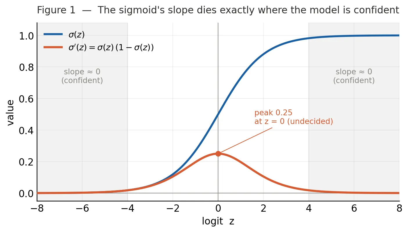
This is the mechanical root of the saturation that Part 1.4 demonstrated with numbers. Recall its worked disaster: the truth was $y = 1$ but the model fed in $z = -6$, so $\sigma(-6) \approx 0.0025$, about as wrong as possible. The slope there is $\sigma'(-6) \approx 0.0025 \times 0.9975 \approx 0.0025$ — almost nothing. We can now see precisely why that number is so small: it is $\sigma(z)(1 - \sigma(z))$ evaluated deep in a flat tail. Whether that near-zero slope poisons the gradient or not depends entirely on the cost function stacked on top, and that is the subject of the next chapter.

---

Chapter 2: The Cost Function That Belongs to the Sigmoid

Take the Negative Log-Likelihood, As Always

We have the output unit from Part 2.1. Now, following the discipline Part 1.3 drilled into us, we do not invent a cost — we take the negative log-likelihood of the distribution we built. For a single example,

$J(\theta) = -\log P(y \mid x).$

There is a subtlety worth confronting directly, because it sounds like a contradiction, and it is the same “predict in log-space” idea from Part 1.3 seen from a new angle. The network’s output, $\hat{y} = \sigma(z)$, genuinely lives in probability space, between $0$ and $1$. So why is the training objective built on a logarithm? Because these are two different places doing two different jobs. The network outputs a probability. The cost takes the log of that probability. Log-space is not a claim about the output; it is where the objective lives — and the reason it lives there is the single most important mechanism in this part.

The Log Undoes the Exponential

We recall from Part 2.1 that we built the sigmoid out of an exponential. When we place a logarithm in the cost, that logarithm reaches into the sigmoid and cancels its exponential. Three small facts assemble the result, so we take them one at a time.

The one-line Bernoulli form. In Part 2.1 the Bernoulli came out in two cases, $P(y=1) = \sigma(z)$ and $P(y=0) = 1 - \sigma(z)$. We pack both into a single expression, using the factor $(2y-1)$ as a switch:

$P(y) = \sigma\big((2y-1)z\big).$

When $y = 1$ the factor is $2(1) - 1 = +1$, so the expression is $\sigma(z)$; when $y = 0$ the factor is $2(0) - 1 = -1$, so the expression is $\sigma(-z)$, which equals $1 - \sigma(z)$. It is the same distribution as before — one line in place of two cases, and that is all “one-line Bernoulli form” means.

The softplus identity. The negative log of a sigmoid is itself a softplus, with the sign of its input flipped:

$-\log \sigma(x) = \zeta(-x), \qquad \text{where } \zeta(x) = \log(1 + e^{x}).$

The proof is three steps, and it leans on two basic logarithm rules: the log of a fraction splits into a subtraction, $\log\frac{a}{b} = \log a - \log b$, and the log of one is zero, $\log 1 = 0$. We expand the sigmoid, split the log of the fraction, and the $\log 1$ term vanishes:

$-\log \sigma(x) = -\log \frac{1}{1 + e^{-x}} = -\big[\underbrace{\log 1}_{=\,0} - \log(1 + e^{-x})\big] = \log(1 + e^{-x}),$

and $\log(1 + e^{-x})$ is exactly $\zeta(-x)$. So taking $-\log$ of a sigmoid turns it into a softplus and flips the sign of the argument — and that sign flip is the whole reason $(2y-1)$ is about to become $(1-2y)$.

Assembling the loss. The full line is now just those two facts applied in order. We start from the maximum-likelihood cost, substitute the one-line form, then apply the identity:

$J(\theta) = -\log P(y \mid x) = -\log \sigma\big((2y-1)z\big) = \zeta\big((1-2y)z\big).$

The last equality is the identity flipping the sign of the argument, since $-(2y-1) = 1 - 2y$. A quick check grounds it: at $y = 1$, $z = 2$ (confident and correct), the direct loss is $-\log\sigma(2) \approx 0.127$, and the softplus form gives $\zeta(-2) = \log(1 + e^{-2}) \approx 0.127$ — the same number, as it must be.

This is the same cancellation that produced squared error from the Gaussian in Part 1.3 — logarithm against exponential — except there it flattened the Gaussian into a clean square, and here it clears the exponential out of the sigmoid so we can write the cost directly in terms of $z$. To see why that matters, we differentiate and compare against squared error, which is exactly the comparison Part 1.4 made numerically and promised to justify here.

Where the Slope Lives, and Where It Doesn’t

The four rules we use, in plain terms. Chain rule: to differentiate a function sitting inside another, we differentiate the outside and multiply by the derivative of the inside — rates multiply along the chain. Power rule: $x^2$ differentiates to $2x$ (bring the power down, subtract one). Log rule: $\log x$ differentiates to $\frac{1}{x}$. Constant rule: a fixed number differentiates to $0$, which is why the true label $y$ vanishes. The chain rule does the main work; the other three handle the pieces it hands back.

This is the heart of the whole part, so we go carefully. Both costs sit on top of the sigmoid, so both must send their correction backward through it, and the chain rule governs that passage. The chain rule says the gradient with respect to $z$ is the derivative of the cost with respect to the output, times the derivative of the output with respect to $z$ — and that second factor is $\sigma'(z)$, the slope we derived in Chapter 1. This is why $\sigma'(z)$ appears in the gradient at all: it is the price of passing through the sigmoid, levied by the chain rule. Part 1.4 asserted this; now we can watch it happen.

Squared error. The cost is $(y - \sigma(z))^2$. Differentiating the outer square gives $-2(y - \sigma(z))$, and the chain rule multiplies by the inner slope $\sigma'(z)$:

$\frac{\partial J}{\partial z} = -2\,(y - \sigma(z))\,\sigma'(z).$

The sigmoid’s slope sits in the gradient as a bare multiplier. When the model is confidently wrong, $\sigma'(z)$ is nearly zero — as we computed, about $0.0025$ at $z = -6$ — and it crushes the whole gradient down to roughly $-0.005$. The correction vanishes precisely when it is most needed. This is saturation, and now we can name its cause exactly: an undefended $\sigma'(z)$ left sitting in the gradient.

Cross-entropy. The cost is $-\log \sigma((2y-1)z)$. Here the logarithm cancels the exponential inside the sigmoid before differentiation, and when the dust settles the $\sigma'(z)$ factor is gone, cancelled rather than multiplied. What remains is startlingly simple:

$\frac{\partial J}{\partial z} = \sigma(z) - y.$

Just “prediction minus truth.” At the same confidently-wrong point, this is $0.0025 - 1 = -0.9975$: a full-strength correction. The gradient is large exactly when the model is wrong and shrinks to zero only when $\sigma(z)$ reaches $y$ — that is, only when the model is right. There is no $\sigma'(z)$ left to sabotage it.

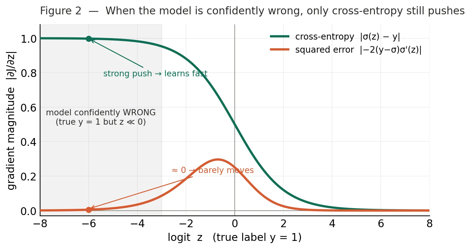
This is the debt from Part 1.4 paid in full. Cross-entropy is not a lucky patch that happens to dodge saturation. It is the derived cost for a Bernoulli output, and the same logarithm that Part 1.3 used to turn products into sums is the one that, here, dissolves the sigmoid’s treacherous slope out of the gradient. We built the output unit and its cost from the same exponential, and they were always meant to cancel.

A Closer Look at the Cancellation

It is worth seeing the cancellation itself, not just its result, because it is the same chain rule on both sides and the outcome still differs. We take the cross-entropy for the $y = 1$ case, $J = -\log \sigma(z)$, and differentiate step by step. The outer $-\log(\cdot)$ contributes $-\frac{1}{\sigma(z)}$, and the chain rule drags in the inner slope $\sigma'(z)$ — exactly as it did for squared error:

$\frac{\partial J}{\partial z} = -\frac{1}{\sigma(z)}\cdot \sigma'(z).$

Now substitute the slope’s derived form, $\sigma'(z) = \sigma(z)\,(1 - \sigma(z))$:

$\frac{\partial J}{\partial z} = -\frac{1}{\sigma(z)}\cdot \sigma(z)\,(1 - \sigma(z)) = -(1 - \sigma(z)) = \sigma(z) - 1.$

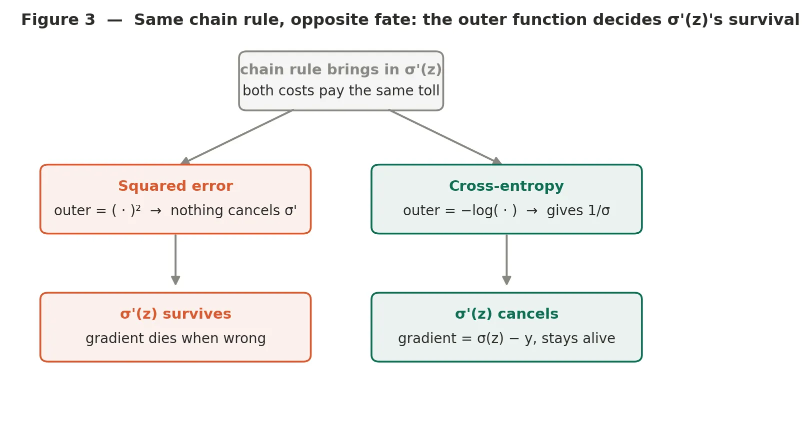
The $\sigma(z)$ pulled in by $\sigma'$ cancels the $\frac{1}{\sigma(z)}$ pulled in by the logarithm — they annihilate, and $\sigma(z) - 1$ is just $\sigma(z) - y$ for $y = 1$. The chain rule drags $\sigma'(z)$ into both gradients; the two costs differ only in their outer function, and that outer function decides the slope’s fate. With the square outside, nothing cancels $\sigma'(z)$ and it survives to kill the gradient. With $-\log$ outside, its derivative produces exactly the $\frac{1}{\sigma(z)}$ that erases $\sigma'(z)$. The pairing is a design, not a coincidence.

Stated as a General Rule

The lesson generalizes past this one case. Whenever our output function is built from an exponential — as the sigmoid is — we pair it with the log-based cost, so the log cancels the exponential and leaves a gradient that stays healthy when the model is wrong. The output function and the cost function are two halves of one design, engineered so that one undoes the other. This is the same conclusion Part 1.4 reached from the cost side; we have now earned it from the output side, with the cancellation shown rather than asserted.

A Small but Real Practical Point

One more reason to keep the cost written in terms of $z$ rather than $\hat{y}$, and it is not theoretical but numerical. Analytically the logarithm of a sigmoid is always well-defined, because the sigmoid returns values strictly inside the open interval $(0, 1)$, never touching the ends. But a real computer has finite precision. If $z$ is very negative, $\hat{y} = \sigma(z)$ can underflow to exactly zero in floating point, and then $\log \hat{y} = \log 0 = -\infty$ ruins the computation — the same underflow danger that motivated the logarithm in Part 1.3, resurfacing from the other direction. Writing the negative log-likelihood directly as a function of $z$, through the softplus form we derived, sidesteps this entirely, because it never forms the fragile intermediate $\hat{y}$. The clean derivation and the stable implementation turn out to be the same expression.

---

Chapter 3: The Unified Picture

One Idea, Two Output Units

We produced both output units across Parts 2.1 and 2.2 by the same discipline Part 1 built, and setting them side by side makes that discipline visible.

Question	Output represents	Output unit	Cost that falls out
A real number?	Mean of a Gaussian	Linear: $\hat{y} = W^{\top}h + b$	Squared error
Yes or no?	Probability of a Bernoulli	Sigmoid: $\hat{y} = \sigma(w^{\top}h + b)$	Cross-entropy

In both rows we never chose the cost by taste. We declared what distribution the output stands for, took the negative log-likelihood of that distribution, and the cost appeared on its own — squared error from the Gaussian, cross-entropy from the Bernoulli. This is the promise of Part 1.3 and 1.4 made concrete at the output layer: the output unit and the cost function are one decision, made once and read off twice.

Why the Sigmoid Was Inevitable

If there is a single thing to carry out of these two parts, it is that the sigmoid was not handed down as a convenient S-shaped curve someone happened to like. A chain of requirements forced it into existence, each one solving the problem the last had left. We needed a probability, so a plain linear number would not do. We wanted that probability from a principle, so we assumed the simplest log-linear form. That assumption produced logs, so we exponentiated for positivity. The scores did not sum to one, so we normalized. Out came the sigmoid and the Bernoulli it parameterizes — and waiting for it, a cost whose logarithm was shaped precisely to cancel the sigmoid’s exponential and keep learning alive, which is why the $\sigma'(z)$ that killed squared error’s gradient never even appears in cross-entropy’s.

The pattern is the one that ran through all of Part 1. Each object exists because the previous one left exactly one thing missing, and each new object is the unique thing that supplies it. The output layer only changes what “missing” means: no longer a direction to step, but a shape for the answer.

---

What Comes Next

We have handled the two-outcome case. But many real problems are not binary — they ask which of many categories an input belongs to, not merely yes or no. A handwritten digit is one of ten classes; a word is one of tens of thousands. Extending the sigmoid to more than two outcomes is not a patch but a natural generalization, and it produces the softmax unit, paired with the same cross-entropy cost, for exactly the same anti-saturation reason we saw here. Running the log-linear-then-normalize derivation with $k$ outcomes instead of two is the whole of it.

The derivation never changes its character. We will state the distribution, take its negative log-likelihood, and let the output unit and its cost fall out together — just as they did here, and just as they did for the Gaussian all the way back in Part 1.3.

---

References

• Goodfellow, I., Bengio, Y., & Courville, A. (2016). Deep Learning. MIT Press. Relevant chapter: Chapter 6 (Deep Feedforward Networks), Section 6.2.2 — Output Units, covering linear units for Gaussian output distributions and sigmoid units for Bernoulli output distributions. Available free at deeplearningbook.org.