The Math Behind Neural Networks, Part 2.1 — Output Units and the Birth of the Sigmoid

A calm, sequential guide for anyone entering the field. The article is divided into smaller chapters to make it easier to understand.

Part 1 built a complete machine and then spent four articles making sure we understood every piece of it. We started with a line, $\hat{y} = wx + b$ , and a hand-picked way to measure its error. We turned that error into learning through the derivative and gradient descent. Then, rather than leave the loss unexamined, we went back and derived it: the mean squared error was not a starting assumption but the consequence of a single principle — maximum likelihood — applied to a single modelling choice, that the output is a Gaussian centred on the prediction. Part 1 closed by reading the menu that principle produces, and it left us standing at a precise edge. The choice of loss and the choice of what the output represents are not two decisions. They are one.

Part 2 begins there. Everything in Part 1 quietly assumed a particular kind of output — a single real number, compared against a single real number. But the last layer of a network does not always produce a plain number. Sometimes it produces a probability. Sometimes a category. And the moment the kind of output changes, the layer that produces it must change too, and the cost that grades it changes along with it. This part is about that last layer specifically — the output units — and about how their form is forced by the distribution we want the output to represent.

Part 1.4 ended by naming exactly what this stretch of the series owes you. It showed, with numbers, that when a sigmoid sits in front of the loss, squared error’s gradient can fall silent at the worst possible moment while cross-entropy’s stays alive. But it deliberately left three things unpaid: where the sigmoid’s slope $\sigma'(z)$ actually comes from, why the chain rule places it inside the gradient, and why cross-entropy is the derived cost for a binary output rather than a lucky patch that happens to work. Part 2 pays those debts across two articles. This one — Part 2.1 — does the first half: it builds the sigmoid from the ground up and watches the Bernoulli distribution produce it, so that by the end we hold the output unit itself and know exactly which distribution stands behind it. Part 2.2 then takes that unit apart — finding its slope by hand, deriving its matched cost, and seeing the cancellation from the inside.

The tools from Part 1 do not change. The forward pass, the loss, the gradient, and the update all still run underneath. What changes is the very last step of the forward pass, and everything that flows from it.

$NN$

Chapter 1: Output Units — Where the Network Meets the Task

The Layer That Finishes the Job

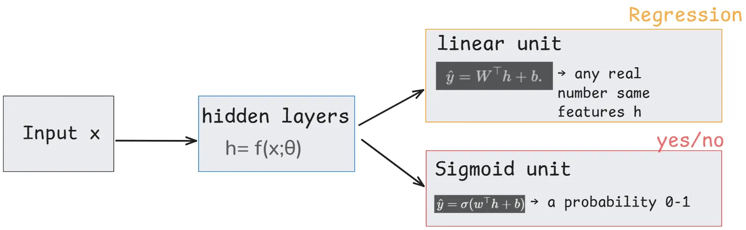
Every network we will study has the same overall shape. The input $x$ enters, and a stack of hidden layers transforms it into a set of learned features. We can write that whole internal process as a single function,

$h = f(x; \theta),$

where $h$ is the vector of features the network has extracted and $\theta$ collects every parameter it learned along the way. Everything up to $h$ is the network understanding the input. What remains is to turn that understanding into an answer of the correct shape. That final turning is the job of the output layer, and the individual neurons that perform it are the output units.

A note on what $f$ really is. Do not read $f(x;\theta)$ as one operation, or as the work of a single neuron. It is an abstraction — a single symbol standing in for the entire stack of hidden layers, however many there are, folded into one name. Inside that box, each layer performs a weighted sum followed by a nonlinearity, and the layers feed into one another in sequence; $f$ simply hides all of that internal machinery so we can talk about the output layer without dragging the whole interior along. The reason we abstract it away is focus: this article is about the last step, so everything before it is compressed into $f$ , and its final result — the feature vector $h$ — is all the output layer ever sees. When you read $h = f(x;\theta)$ , read it as “let $h$ be whatever the hidden part of the network produced,” and nothing more.

It is worth being exact about a word here, because it is a common source of confusion. An output unit is not a different species of object from the neurons inside the network. A unit is a single neuron: it takes a weighted sum of its inputs and applies some function to the result. A layer is a group of such units. The output layer is simply the last group — the one whose result is not passed any deeper but handed back as the network’s answer. What makes an output unit an output unit is its position, not its nature.

That observation carries a principle worth holding onto. Any function that can serve at the output can also serve inside the network as a hidden unit, because it is the same kind of building block either way — the only difference is whether its result is the final answer or an intermediate feature passed further along. The same sigmoid that produces a final probability at the output can sit buried in a hidden layer adding nonlinearity. Same function, different job. For this article the output position is the one that matters, because that is where the function is chosen to match the task.

The Choice of Output Determines the Cost

Part 1.3 and 1.4 built one idea carefully, and it is the hinge for everything below, so it is worth restating in one line. The cost function is not something we design by hand. It is handed to us, the moment we decide what distribution the model’s output represents. Choose the output to be the mean of a Gaussian, and the negative log-likelihood is squared error — that was the whole payoff of Part 1.3. Choose it to be the probability of a yes-or-no event, and the negative log-likelihood is the cross-entropy whose gradient we watched survive the sigmoid in Part 1.4.

So the output unit and the cost function are chosen together, as one matched pair. Part 1 established this from the side of the cost. This part establishes it from the side of the output — we will pick a distribution, and watch both the output unit and its cost fall out together. Every chapter below is an instance of that single move.

Chapter 2: Linear Units — The Mean of a Gaussian

The Simplest Possible Output

The gentlest output unit is the one that applies no nonlinearity at all. Given the features $h$ , a layer of linear output units produces

$\hat{y} = W^{\top} h + b.$

That is the whole thing: an affine transformation, a weighted sum plus a bias, with nothing wrapped around it. Because there is no squashing function, the output is free to be any real number, positive or negative, large or small. This is exactly what you want when the quantity you are predicting is itself an unbounded real number — a temperature, a price, a length.

A short note on the notation, because it genuinely trips people up. You will see both a capital $W$ and a lowercase $w$ in these formulas, and it is tempting to guess that capital means “hidden layer” and lowercase means “output layer.” That guess is wrong. The rule is about the shape of the output, not the position in the network. A capital $W$ is a matrix, used whenever the layer produces a vector of several numbers. A lowercase $w$ is a vector, used whenever the layer produces a single scalar. In the linear layer above, $\hat{y}$ is bold because it is a vector — several predicted numbers at once — so the weights form the matrix $W$ . When a layer collapses everything to one number, it uses $w$ , and the transpose is the tell: $W^{\top}h$ is matrix-times-vector and yields a vector, while $w^{\top}h$ is a dot product and yields a single scalar.

$NN$

Why This Is Secretly the Gaussian From Part 1.3

On the surface a linear output unit has nothing to do with probability; it just computes a number. But the reason it pairs with squared error is exactly the derivation Part 1.3 already carried out, now read from the output side. We treat the network’s output not as a flat prediction but as the mean of a Gaussian over the true target,

$p(y \mid x) = \mathcal{N}(y;\ \hat{y},\ I).$

Given the input, the target is modelled as normally distributed, centred on whatever the network predicted, with a fixed spread. The network’s only job is to move that centre to the right place. It is worth being exact about the direction here, because it is easy to picture backwards: the network does not lay down a bell curve and then pick its highest point as the answer. It is the reverse. The network computes the number $\hat{y}$ directly, straight out of $\hat{y} = W^{\top} h + b$ , and that number is the prediction; the bell curve is then drawn around it, with its peak sitting on $\hat{y}$ by construction. So “near $\hat{y}$ ” is not a value we read off a pre-existing curve — the curve exists because the network produced $\hat{y}$ , and training slides the peak toward the truth by changing $\hat{y}$ itself, through the weights $W$ and bias $b$ . Notice, in passing, that $\hat{y}$ is a vector here — the mean vector — and the covariance is the identity matrix $I$ ; the fact that the covariance is a matrix is itself why the weights producing $\hat{y}$ must be the matrix $W$ . The notation is consistent once you read it as a statement about dimensionality.

A note on the two ways to write a layer. The same matrix-vs-vector logic explains the layer that produced $h$ in the first place, and it is worth seeing the two forms side by side, because they are the same thing at two zoom levels. Zoom in on a single hidden layer of, say, ten neurons, and each neuron computes its own weighted sum with its own weight vector and bias, then applies the activation $g$ :

$h_1 = g(w_1^{\top} x + b_1), \quad h_2 = g(w_2^{\top} x + b_2), \quad \dots, \quad h_{10} = g(w_{10}^{\top} x + b_{10}).$

Ten neurons, ten separate formulas, ten output numbers — and crucially they run in parallel, each with different weights, so each detects a different feature rather than repeating the same one. Those ten numbers are then stacked into the feature vector $h = [\,h_1, h_2, \dots, h_{10}\,]^{\top}$ . Now zoom out: stack the ten weight vectors $w_1, \dots, w_{10}$ as the rows of one matrix $W$ , and all ten formulas collapse into a single line,

$h = g(Wx + b).$

This is why the matrix appears — it is simply the compact way to write “many neurons, each doing its own weighted sum, all at once.” So $h$ is a vector (one slot per neuron), $W$ is the matrix that holds every neuron’s weights, and the per-neuron form and the packed matrix form describe the identical computation. The matrix form is what lives, layer after layer, inside the abstract $f(x;\theta)$ from Chapter 1.

We do not need to redo the algebra — Part 1.3 took the negative log-likelihood of this Gaussian, the logarithm cancelled the exponential, the constants fell away, and what survived was $\tfrac{1}{2}\lVert y - \hat{y}\rVert^2$ , the squared error. The point to carry forward is the shape of that move, because we are about to run it a second time. State the distribution, take the negative log of its likelihood, and the cost appears on its own. The linear unit is the first and simplest instance: an output with no nonlinearity, married to squared error, because its distribution is a Gaussian whose mean it predicts.

Chapter 3: The Problem That Forces a New Output Unit

When the Answer Is Yes or No

The linear unit handles unbounded real numbers. But an enormous class of problems does not ask for a real number at all. They ask a binary question. Is this email spam or not? Does this image contain a cat? Will this customer churn? The target $y$ is not a temperature; it is a single bit, $y \in \{0, 1\}$ .

We could try to force the linear unit onto this problem — let it output a number and call anything above $0.5$ a “yes.” It fails, and the failure has two layers worth separating, because the second is far deeper than the first.

The first failure is the range. A probability must live between $0$ and $1$ , but a linear unit produces any real number it likes — $-4$ , $17.3$ , anything at all. A prediction of $17.3$ for “the probability this email is spam” is not merely untidy; it is meaningless, and there is no honest way to read it as a confidence. On this reading the output is simply the wrong shape for the question — it lands outside the only range a probability is allowed to occupy.

The second failure is deeper: the distribution itself is wrong. Recall from the previous chapter that using a linear unit with squared error is secretly assuming a Gaussian over $y$ . So look hard at what that Gaussian actually claims. It is a bell curve stretching to infinity in both directions, asserting that the answer could plausibly be near $0.5$ , or $2$ , or $-3$ , or $40$ , with smoothly tapering probability on every side. That is a faithful description of a temperature. It is an absurd description of a yes/no answer, where the only two values that can ever occur are exactly $0$ and exactly $1$ — nothing between them, nothing beyond them. The Gaussian here is not slightly miscalibrated; it is describing a world that does not match the data at all. This is what it means for the model and the data to be in open contradiction: the bell curve believes in a whole continuum of possible answers, while reality only ever hands us two. Fixing the range without fixing this would be treating a symptom — the real error is that we chose the wrong distribution before we ever chose the output unit.

$NN$

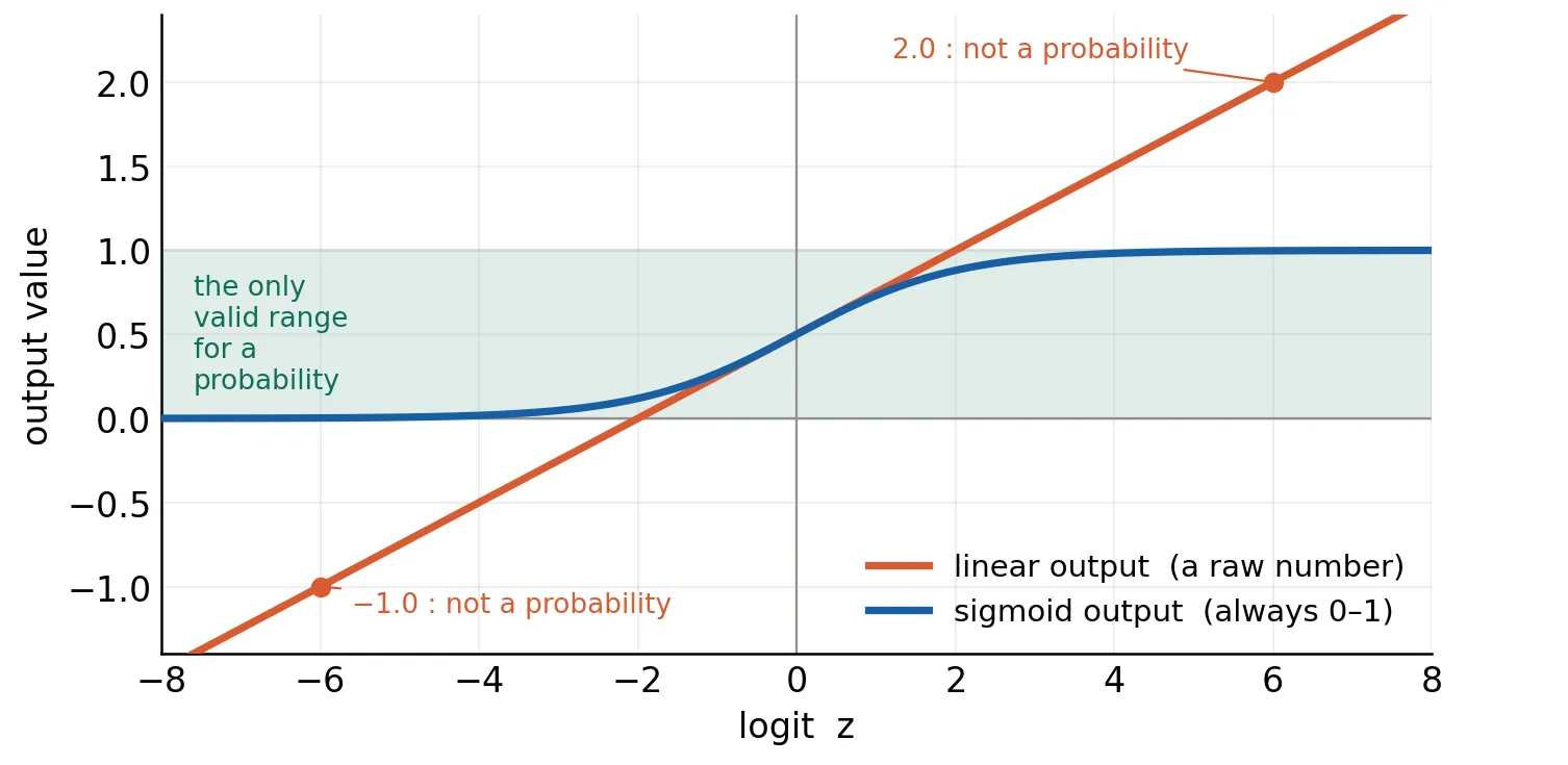
What we need, then, is a new kind of output unit built on a distribution that actually fits the situation: not a continuous bell curve over an infinite range, but a distribution over exactly two outcomes. Its result must always be a valid probability — a number squeezed into the open interval between $0$ and $1$ — that we can read as the probability the answer is “yes.” That two-outcome distribution has a name: the Bernoulli, the mathematics of a single (possibly unfair) coin flip — one probability $p$ for “yes” and $1-p$ for “no,” and nothing in between.

Part 1.4 already showed us the output unit that turns a raw score into exactly this — the sigmoid — and used it to expose the saturation problem. But it pulled the sigmoid out of the air as a given, deferring the real question to here. This chapter and the next answer it properly: not that the sigmoid works, but why it must be the sigmoid — deriving both it and the Bernoulli it produces from a single honest assumption, rather than accepting them as gifts.

Chapter 4: Deriving the Sigmoid Unit

The Two-Part Structure

A sigmoid output unit is built in two stages, and keeping them separate makes everything clearer. First, exactly as in the linear case, a layer computes a single real number:

$z = w^{\top} h + b.$

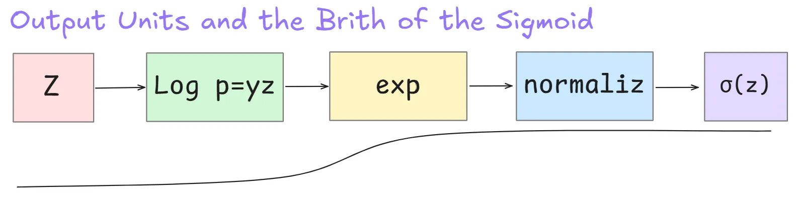
This number $z$ is unbounded — the same kind of raw score the linear unit produced. It has a name: the logit. Second, we pass $z$ through a function whose entire purpose is to convert that unbounded score into a probability. That function will turn out to be the sigmoid, $\sigma$ . The linear part does the learning; the sigmoid part does the squashing. Our task is to discover what that squashing function must be, if we insist it produce a proper probability from a principle rather than a patch.

$NN$

Why Start in Log-Space?

Before we assume anything, it is worth answering the question a careful reader asks right here: why bring in a logarithm at all? Why not just set the linear score equal to the probability directly and be done?

The answer is a mismatch of ranges, and it is the reason for everything that follows. Our linear tool is comfortable and familiar — $z = w^{\top} h + b$ — but by its nature it can produce any real number, from $-\infty$ to $+\infty$ . A probability is the opposite kind of thing: it is trapped between $0$ and $1$ . So the naive move, writing

$P(y = 1) = z,$

is broken on arrival. It sets a bounded quantity equal to an unbounded one. When $z$ comes out as $12$ , or as $-5$ , this equation is claiming the probability is $12$ or $-5$ — which is meaningless. You cannot equate something that must stay inside $[0, 1]$ with something free to run off to infinity; the two sides do not even live in the same range.

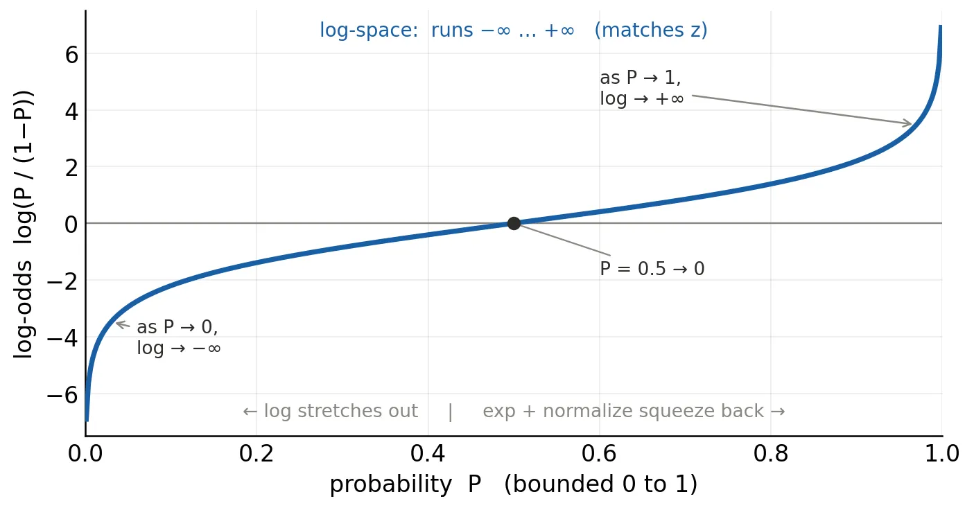
There are two ways to reconcile the ranges. You could try to crush $z$ down into $[0, 1]$ — but that fights the linear layer’s whole nature. The cleaner move is the reverse: stretch the probability up to meet $z$ . And that is exactly what the logarithm does. Feed it a value in $(0, 1)$ and it hands back a value spanning the entire real line: as the probability rises toward $1$ , its logarithm climbs toward $0$ ; as the probability falls toward $0$ , its logarithm plunges toward $-\infty$ . So $\log P$ ranges over all of $(-\infty, +\infty)$ — precisely the range $z$ already lives in.

Now the two sides fit. We can honestly place our linear expression on the log side of the equation, because both sides can now reach the same values. This is why the assumption in the next section is written about $\log \tilde{P}(y)$ rather than about $P(y)$ directly: log-space is the one place where the unbounded linear score and the (transformed) probability can be set equal without breaking any rule.

One worry to head off, because it sounds like a contradiction. If the whole problem was that a probability must not be unbounded, why is it suddenly fine — even desirable — to send it out toward $\pm\infty$ with a logarithm? Because the danger was never “unbounded numbers exist.” The danger was the mismatch — equating a bounded thing with an unbounded one. Log-space is not where we leave the answer; it is a temporary bridge. We do the linear work there, and then, in the next two steps, the exponential and the normalization carry everything back down into the safe $(0, 1)$ range where a probability belongs. The logarithm is a translator, not a risk: it lets the linear equation and the world of probabilities understand each other, and once they have, we translate back.

One Honest Assumption

We are going to build a probability distribution over $y \in \{0, 1\}$ starting from the single number $z$ . Rather than guessing the shape of the probability directly, we make an assumption about the logarithm of an unnormalized probability — a set of positive scores that need not sum to $1$ yet, which we will normalize afterward. The assumption is the simplest one available: that this log-probability is linear in $y$ and $z$ together. Concretely,

$\log \tilde{P}(y) = yz.$

“Linear in $y$ and $z$ ” means literally that the expression is the product $y \times z$ — no squaring, no higher powers, no trigonometry, just the simplest possible interaction between the two quantities. And this simplest choice is not made blindly; it does exactly what we want. Since $y$ is either $0$ or $1$ , substitute both cases and watch:

when $y = 1$ , the log-score is $\log \tilde{P}(1) = z$ ;
when $y = 0$ , the log-score is $\log \tilde{P}(0) = 0$ .

The single number $z$ now directly controls the log-score of the “yes” class, while the “no” class sits pinned at zero as a fixed reference. This is precisely what we want from a logit: one knob that pushes the two outcomes apart.

Why Exponentiate

We assumed a form for the logarithm of the score, so to recover the score itself we undo the logarithm — and the inverse of the logarithm is the exponential. Applying $\exp$ to both sides gives

$\tilde{P}(y) = \exp(yz).$

This is one algebraic step, not a trick. But there is a deeper reason the exponential is the natural choice and not merely the mechanical one. Probabilities must be positive, always, and the exponential returns a positive value for every input, however large or negative. Whatever $z$ turns out to be, $\exp(yz)$ is guaranteed to be a valid positive unnormalized score. The exponential is the bridge that carries an unbounded logit into the world of positive numbers. (Keep this exponential in view — in Chapter 6 the logarithm inside the cost is going to reach back in and cancel it, and that cancellation is the entire reason the sigmoid trains well.)

Normalizing into a Distribution

We now have two positive scores, one per outcome, but they need not sum to $1$ , so they are not yet a distribution. We fix that the only way one can: divide each score by the total. This is normalization.

$P(y) = \frac{\exp(yz)}{\sum_{y'=0}^{1} \exp(y'z)} = \frac{\exp(yz)}{\exp(0) + \exp(z)} = \frac{\exp(yz)}{1 + \exp(z)}.$

Write out both outcomes explicitly:

$P(y=1) = \frac{\exp(z)}{1 + \exp(z)} = \sigma(z),$

$P(y=0) = \frac{1}{1 + \exp(z)} = 1 - \sigma(z).$

Two things arrive at once, and both deserve a moment.

First, the probability of the “yes” class came out exactly equal to $\sigma(z) = \frac{1}{1 + e^{-z}}$ , the sigmoid. (The two forms are the same: multiply numerator and denominator of $\frac{e^z}{1+e^z}$ by $e^{-z}$ .) We did not assume the sigmoid and check that it behaves — we assumed linearity in log-space and the sigmoid fell out as the forced consequence. This is the answer to the question Part 1.4 deferred: the sigmoid is where it is because it is what “linearity in log-space, exponentiated, then normalized” is. It is a result, not a starting point.

Second, we produced a distribution over a single binary variable, with probability $\sigma(z)$ for one outcome and $1 - \sigma(z)$ for the other. That, by definition, is a Bernoulli distribution — the distribution of any yes/no event, a single coin flip with a possibly unfair coin. This is why these are called sigmoid units for Bernoulli output distributions: the sigmoid is the machine, and the Bernoulli is what it produces. There is nothing more exotic to a Bernoulli than “one probability $p$ and its complement $1 - p$ ,” and here $p = \sigma(z)$ .

The book compresses both outcomes into one tidy line,

$P(y) = \sigma\big((2y-1)z\big),$

worth decoding once so it does not look like magic. Put $y = 1$ and the argument becomes $z$ , giving $\sigma(z)$ . Put $y = 0$ and the argument becomes $-z$ , giving $\sigma(-z)$ , and a basic identity of the sigmoid is $\sigma(-z) = 1 - \sigma(z)$ . The one-line form is not a new fact; it is the two cases we already derived, folded together.

The Full Derivation at a Glance

It helps to see the whole chain in one place, because each step exists only to repair the specific defect the previous one left behind — the same style of reasoning that ran through Part 1.

Step	Expression	Problem it solves
Logit	$z = w^{\top}h + b$	Produces a raw score, but it is unbounded
Linear assumption	$\log \tilde{P}(y) = yz$	Fixes the log-score cleanly, but it is a log, not a probability
Exponentiate	$\tilde{P}(y) = \exp(yz)$	Forces positivity, but the scores do not sum to one
Normalize	$P(y) = \dfrac{\exp(yz)}{1 + \exp(z)}$	Forces a valid distribution
Result	$P(y = 1) = \sigma(z)$	A sigmoid, and a Bernoulli, derived rather than assumed

Nothing in the table was invented for convenience. Each row is the unique repair for the defect in the row above it.

What Comes in Part 2.2

We have the sigmoid now, and we never had to assume it. Starting from a single honest assumption — that the log of an unnormalized probability is linear in $y$ and $z$ — we exponentiated for positivity, normalized into a distribution, and watched the sigmoid and the Bernoulli it parameterizes fall out as forced consequences rather than gifts. The output unit for a yes-or-no question is built, and we know exactly which distribution stands behind it.

But building the unit is only half the story. We have the shape of the sigmoid without yet knowing how it behaves when training pushes on it — and that behaviour is where the debts from Part 1.4 finally come due.

Part 2.2 pays them. It begins with the sigmoid’s slope, $\sigma'(z)$ — the quantity Part 1.4 slipped into the gradient through the chain rule and asked you to accept on faith. We derive it by hand, find that it collapses to the elegant $\sigma(z)\,(1 - \sigma(z))$ , and see why that form is the mechanical root of saturation: the slope dies precisely where the sigmoid goes flat. Then we do for the Bernoulli what Part 1.3 did for the Gaussian — take the negative log-likelihood and let the cost appear on its own. This time the logarithm reaches into the sigmoid and cancels the very exponential we built into it in this part, and out of that cancellation comes the reason cross-entropy’s gradient stays alive exactly where squared error’s falls silent. The saturation that Part 1.4 could only show you with numbers, Part 2.2 will explain from the inside.

The output unit and its cost were made from the same exponential, and they were always meant to meet. This part built the first half. The next part lets them meet.

References

Goodfellow, I., Bengio, Y., & Courville, A. (2016). Deep Learning. MIT Press. Relevant chapter: Chapter 6 (Deep Feedforward Networks), Section 6.2.2 — Output Units, covering linear units for Gaussian output distributions and sigmoid units for Bernoulli output distributions. Available free at deeplearningbook.org.