The Math Behind Neural Networks, Part 1.4 — Which Loss to Choose, and Why
Aug 18, 2026
A calm, sequential guide for anyone entering the field. The article is divided into smaller chapters to make it easier to understand.
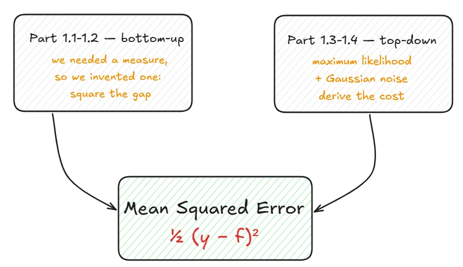
Part 1.3 ended on a quiet victory. The mean squared error, which we had simply assumed back in Part 1.1 and optimised in Part 1.2, was no longer an assumption. We had derived it — from a single principle, maximum likelihood, and a single modelling choice, that the model’s output is a Gaussian centred on its prediction. The loss we had trusted for two parts was finally standing on a foundation we could see through. The recipe was built: choose the output distribution, and the cost follows.
But a recipe that produces one dish invites an obvious question about all the others. We chose the Gaussian, and squared error came out. That was a choice — the introduction to Chapter 9 said as much and then set the point aside. This part picks it back up. If a different output distribution is chosen, a different cost comes out, and it predicts a different summary of the data. Squared error was never the only item on the menu; it was the first one we happened to order.
There is also a problem hiding inside the loss we derived, one that Part 1.3 had no reason to expose. In the very common case of a yes-or-no prediction, squared error can go quiet at exactly the wrong moment — its gradient falling nearly to zero while the model is still confidently wrong, leaving gradient descent with nothing to follow. The fix is not to patch squared error but to derive a different cost, cross-entropy, from a different distribution, and watch the problem dissolve on its own. This is where the slope idea from Part 1 returns for the last time, and where the choice of loss and the choice of output finally reveal themselves as one decision, not two.
So this part is about reading the menu that Part 1.3 built. We look at what other distributions give, why the loss you pick quietly decides which statistic your model chases, and why practitioners so often reach past the squared error we worked so hard to justify.
Chapter 10: When the Gradient Lies
We built the general recipe, and we chose the Gaussian, and squared error came out. So we could stop. But the practitioners’ literature contains a quiet recommendation that seems, at first, to contradict everything we just did: for many problems, do not use squared error. Use cross-entropy instead. This chapter explains why, and the explanation reaches all the way back to the slope idea from Part 1.
What Is Actually Being Compared
Putting squared error next to cross-entropy can look like a category mistake, so it is worth being clear about what is being compared. They are the same kind of object — both are cost functions, both are numbers measuring how wrong the model is, both are handed to us by the recipe once we pick an output distribution (Gaussian gives squared error; the binary distribution we will meet in Part 2 gives cross-entropy). So comparing them is fair. The reason they come into conflict is not the costs themselves. It is what sits in front of them.
The conflict appears in a specific and very common situation: a binary classification task, where the model must output a yes-or-no probability. To produce a number between 0 and 1, the output is almost always passed through a sigmoid first. And it is the sigmoid, wedged between the network and the cost, that causes the trouble. As we will see, the sigmoid has flat regions, and when squared error is stacked on top of a sigmoid, those flat regions leak into the gradient and flatten it too. During back-propagation — the backward pass we built in Part 1.2 and will extend across layers later — a flat gradient means the update is negligibly small, so the model barely changes even when it is badly wrong. Cross-entropy is the cost whose shape cancels that flattening. That is the whole subject of this chapter: not “which cost is better in the abstract,” but “which cost survives contact with the sigmoid.”
One note before the mechanics. Below, a term written σ′(z) will appear — the slope of the sigmoid. Do not worry about where it comes from in detail here; it is simply the sigmoid’s own steepness at a point, and it enters through the chain rule exactly as the slope did in Part 1.2. We are using it only to see the effect. The full story of the sigmoid, its slope, and the binary (Bernoulli) distribution that makes cross-entropy the derived cost for this task belongs to Part 2.1, where output units are the main subject. Here we only need to watch what σ′(z) does to the gradient.
Two Reasons a Gradient Can Be Small
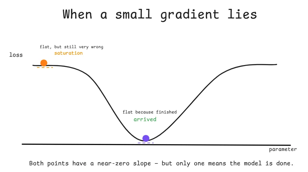
Recall from Part 1.2 that training lives or dies by the gradient. If the slope of the loss goes flat, gradient descent has nothing to follow and learning stalls, like standing on a flat plateau in fog with no sense of which way is downhill.
Now here is the subtlety. A gradient can go small for two completely different reasons, and only one of them is benign.
The first is the good kind. In your worked example in Part 1.2, as w approached its true value of 2, the errors shrank and the gradient shrank with them. A small gradient there means you have essentially arrived — take smaller steps. Nothing is wrong.
The second is the disaster. The gradient can go nearly to zero while the model is still badly wrong. When this happens, the small gradient is lying: it whispers “nothing to fix here” at exactly the moment the model is confidently mistaken and most needs a shove. This second case has a name. It is called saturation, and avoiding it is the reason cross-entropy is preferred.
Where Saturation Comes From, With Numbers
To see saturation appear, we need an output that can be confidently wrong. Binary outputs are the clean example, and this is exactly the setting flagged above: the model must answer yes-or-no, so it produces a probability through a sigmoid, a function that squashes any number z into the range 0 to 1:
The sigmoid is steep in the middle and flat at both ends. Those flat ends are where saturation lives. Set up the disaster: the true answer is y = 1, but the model feeds in a large negative z = −6, confidently insisting the answer is 0.
The model is as wrong as it is possible to be. A good cost function must respond with a large gradient — a hard correction, so that back-propagation actually moves the weights. Watch what each cost does when it has to send that correction back through the sigmoid.
Squared error. To send a correction backward, the chain rule forces the sigmoid’s own slope σ′(z) into the gradient as a multiplier — the backward pass has to pass through the sigmoid, and passing through it means multiplying by its steepness. That steepness obeys σ′(z) = σ(z)(1 − σ(z)), which at z = −6 is 0.0025 × 0.9975 ≈ 0.0025 — almost nothing. (Why σ′ appears here at all, and why it takes this exact form, is the chain-rule story we will tell properly in Part 2.1; for now, watch its effect.) That near-zero slope multiplies into the whole gradient and crushes it:
A shove of −0.005 is no shove at all. The model is maximally wrong, and squared error tells it to barely move. During back-propagation that update is negligible — the weights hardly change. That is saturation, made concrete.
Cross-entropy. Now use the cross-entropy cost, −log σ(z), for the same wrong prediction. Its gradient collapses, through the same cancellation of logarithm against exponential that produced squared error from the Gaussian back in Chapter 9 — only this time the cancellation works for us. The sigmoid’s slope σ′(z) vanishes from the expression entirely, leaving
A shove of about −1: strong, decisive, exactly what a maximally wrong model deserves.
The Whole Argument in One Table
For the identical confidently-wrong prediction — truth 1, model saying 0.0025 — the two costs behave as differently as possible:
| cost | gradient (the shove) | what it says |
|---|---|---|
| Squared error | ≈ −0.005 | ”barely move” |
| Cross-entropy | ≈ −0.9975 | ”move hard, fix this now” |
Same mistake, a roughly two-hundred-fold difference in the correction. The reason is a single mechanical fact. Squared error leaves the output function’s own slope σ′(z) sitting inside the gradient as a multiplier, and that slope dies in the flat regions — so squared error’s gradient dies exactly when the model is confidently wrong. Cross-entropy’s logarithm cancels that slope before it can do damage, keeping the gradient alive no matter how far out the model has wandered.
This is what the recommendation means when it says cross-entropy is preferred even when you do not need a full probability distribution. It is not, at bottom, a statement about probabilities. It is a statement about keeping the slope from Part 1 alive, so that the gradient descent of Part 1.2 always has something real to follow.
Chapter 11: Learning a Single Statistic
There is one more idea in this territory, and it is worth stating for completeness, though we will hold it lightly because its machinery is not needed for anything ahead.
Sometimes we do not want the whole distribution over y. We want just one summary number about it — most often its average. A single summary number like the mean is called a statistic, and there is a way to design a cost so that the trained model chases exactly the statistic we want.
The formal results here are proved with a tool called the calculus of variations, which optimizes over whole functions rather than over a finite list of parameters. You do not need that tool, and we will not use its equations. What you should carry away is the single sentence they establish: the cost function you choose secretly decides which statistic the model predicts.
Concretely, minimizing squared error drives the model toward the mean of y at each input, while minimizing the absolute error |y − f(x)| drives it toward the median. That is the entire practical content. It explains, for instance, why you might prefer absolute error when your data has outliers: the mean gets dragged around by extreme values, and the median does not. It also puts the absolute value in its proper place. Part 1.1 set it aside as a training loss because of the corner at zero that confuses gradient descent — and that objection still stands. But that was never a claim that the absolute value is meaningless; it is the honest maximum-likelihood cost for a particular output distribution (the Laplace), and it targets the median. So the two articles agree: the absolute value is a legitimate cost with a clear statistical meaning, and it is simply awkward to optimize, which is why we reach for it only when its robustness to outliers is worth the trouble. Hold this as a plain fact. The proof behind it is optional and belongs to a later, more theoretical chapter.
Chapter 12: The Unified Picture
How All Concepts Relate
Every step in this part was answering the same question: given that a model is uncertain, how do we measure — and then minimize — how badly its uncertainty misses the truth? The complete chain looks like this:
| Concept | What It Does | The Question It Answers |
|---|---|---|
| Output distribution | Model outputs a spread of belief, not a point | How confident is the model, and in what? |
| Maximum likelihood | Reward high probability on real data | What makes one model better than another? |
| Multiply probabilities | Combine per-example probabilities into one | How well does the model explain all the data at once? |
| Negative log-likelihood | Turn the product into a stable sum to minimize | How do we compute that without underflow? |
| Cross-entropy | Another name for the same quantity | (identical idea, standard vocabulary) |
| Gaussian choice → MSE | Derive squared error from the recipe | Where did the mean squared error come from? |
| Saturation / cross-entropy | Keep the gradient alive when confidently wrong | Why prefer cross-entropy over squared error? |
| Cost decides the statistic | Squared → mean, absolute → median | Which summary of y does the model chase? |
The Reasoning Loop in Plain Language
A cost function, in this view, is never invented by hand. It is derived by four moves. First, decide what distribution the model outputs — a statement about the data, not about your taste. Second, ask for the probability that distribution assigns to the answers that really occurred. Third, take the negative logarithm so the product of those probabilities becomes a stable sum you can minimize. Fourth, if the output function can saturate, prefer the form of the cost whose logarithm cancels that saturation, so the gradient never goes quiet while the model is still wrong.
The model never knows the correct distribution in advance. It starts uncertain in the wrong way, is scored by how much probability it gave to the truth, and is nudged by the very gradient descent of Part 1.2, toward giving more. Everything we built earlier still runs underneath. We have only replaced the hand-picked loss at the top with one we can now justify from first principles.
What Comes in Part 2.1
We have decided how to measure a model’s wrongness, and we have seen that the measurement is tightly bound to what the model’s output represents — a mean, a probability, a category. That binding is the subject of the next part.
Part 2.1 turns to the output units themselves: the last layer of the network, and how its form must be matched to the cost. We will see why a plain linear output pairs with the Gaussian and squared error, why a sigmoid output pairs with binary cross-entropy through the Bernoulli distribution, and how the softmax generalizes this to many categories. That is also where we settle the debts left open in Chapter 10: where the sigmoid’s slope σ′(z) comes from, why the chain rule places it in the gradient, and why cross-entropy is the derived cost for a binary output rather than a lucky fix. The recurring theme will be the one this part uncovered — that the choice of output unit and the choice of cost are not two decisions but one, because the cost is derived from the output distribution, and saturation is avoided only when the two are chosen together.
The slope equation never changes. We are simply learning, layer by layer, what it is measuring.
Refrences
- Goodfellow, I., Bengio, Y., & Courville, A. (2016). Deep Learning. MIT Press. Relevant chapter: Chapter 6 (Deep Feedforward Networks), Section 6.2.1 — Cost Functions. Available free at deeplearningbook.org.