The Math Behind Neural Networks, Part 1.3 — Where the Loss Function Comes From

A calm, sequential guide for anyone entering the field. The article is divided into smaller chapters to make it easier to understand.

Part 1.2 left us with a working method but an unexamined assumption. We had a loss, the mean squared error, and we had turned it into a training procedure through the derivative and gradient descent. We watched the loss fall from 18.67 to 0.297 in a single step and then converge to the true relationship in the data. Everything worked. But we never asked where the mean squared error itself came from. We wrote it down as a reasonable way to measure error — square the gap, average it — and moved on. Because it worked, the question never surfaced.

Look again at how it entered. In Part 1.2, the model gave us a form for the line, ŷ = wx + b, but no way to judge whether a particular guess of w and b was any good. The equation described the model and contained no built-in measure of its quality. Faced with that gap, the article said, in as many words: “So we invented one.” We compared the prediction to the truth across all the data and summarised the gap into a single number. Squaring came along because it was reasonable — it makes every error positive and punishes large misses — not because anything forced it.

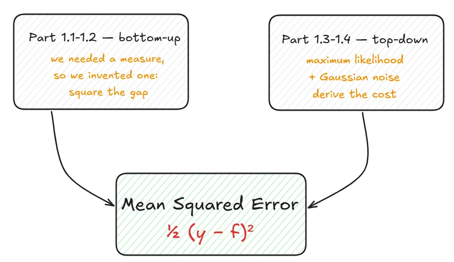
This part is about where that invention actually came from. Why squared error, and not the plain distance, or the cube? The honest answer is that the mean squared error is not a starting point at all. It is a consequence. It is what you are forced to when you begin from a deeper and more general principle about what it means for a model to be good. In this part we start from that principle, watch it produce a single general recipe for building cost functions, and then watch the mean squared error fall out of that recipe on its own.

Readers of Part 1.1 were promised this. Its closing note mentioned, almost in passing, that minimising the mean squared error is equivalent to maximum likelihood estimation under the assumption of Gaussian noise. That sentence was a debt. This part pays it: everything below is the unpacking of that one line. Part 1.4 then asks the next question — whether the loss we just derived is the one we should actually use.

$NN$

Chapter 7: What a Cost Function Really Measures

A Note on Three Names

At the end of Part 1.2 we had a complete loop: predict, measure the loss, compute the gradient, take a step. The loss at the centre of that loop was

$L = \frac{1}{n} \sum_{i=1}^{n} (y_i - \hat{y}_i)^2$

A quick word on names first, because this article introduces a third one and I do not want it to look like a third thing. In Part 1.1 we called this the error function. In Part 1.2 we called it the loss. In this part, and in most textbooks, you will also see it called the cost function, written J(θ). These are not three different objects. They are three names for the same idea — a single number that measures how wrong the model is and that training tries to make small. “Cost function” is simply the more general term the literature settles on once the measure is no longer tied to one particular formula, which is exactly the situation this article is about to put us in. Wherever you read “cost” below, you may read “error” or “loss” and lose nothing.

The Assumption We Never Examined

With the naming settled: as the introduction recalled, this measure entered the story as an invention — the reasonable thing we reached for when the model gave us no measure of its own quality. Squaring makes every error positive, so overshooting and undershooting both count as wrong, and it punishes a large miss far more than a small one. These are good properties, and they were enough to justify the formula for a first encounter.

But “good properties” is not the same as “forced.” An invention fills a gap; it does not prove it was the only thing that could have filled it. A reader who accepts squared error should be able to answer the harder question that the invention quietly left open: out of all the ways to measure a gap, why this one? Some of that question we have in fact already answered. In Part 1.1 we asked the most natural competing question — why not the absolute gap |y − ŷ|, which also removes the sign — and we ruled it out for a concrete reason: the absolute value has a sharp corner at zero where its slope jumps from −1 to +1 with no value in between, and gradient descent, which lives or dies by reading a clean slope, receives contradictory signals at exactly the point it is trying to settle into. So the absolute value is not an open door; Part 1.1 already closed it, on grounds of the slope.

What Part 1.1 did not close is the deeper question. Ruling out the absolute value tells us squaring is better-behaved than one rival. It does not tell us that squaring is right — that out of every smooth, well-behaved measure we could have invented, this is the one the problem actually calls for. For that we need to stop justifying squared error from the outside and find the principle that produces it from the inside. This chapter goes looking for that principle.

From a Point Guess to a Distribution

In Part 1.2, the model produced a single number: ŷ = wx + b. Given an input, it committed to one answer. This is the natural picture, and it is also the picture that hides the principle we are looking for.

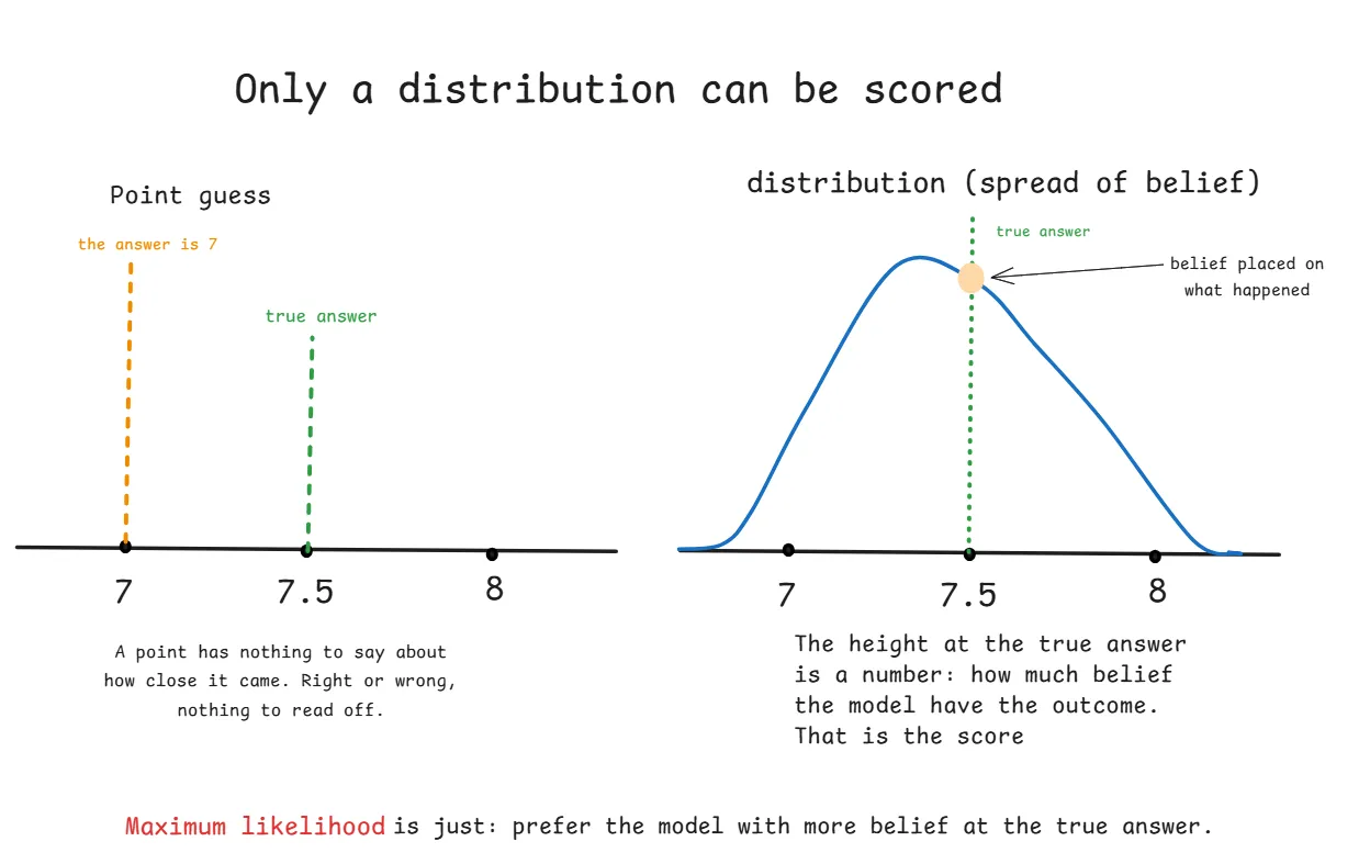
The more honest picture is this. A model is uncertain. Given an input x, it does not truly believe the answer is exactly one number. It believes the answer is probably near some number, with smaller and smaller chances the further you move away. In other words, the model does not output a point. It outputs a distribution — a spread of belief over all the answers that could occur. We write this distribution as

$p_{\text{model}}(y \mid x; \theta)$

read as “the probability the model assigns to the answer y, given the input x and the current parameters θ.” Instead of saying “the answer is 7,” the model says “there is a high chance the answer is near 7, a smaller chance it is 6 or 8, and almost no chance it is 100.”

This is not a complication for its own sake. It is the move that unlocks everything, because once the model outputs probabilities, we can finally ask a precise question about whether it is any good: did the answers that actually happened receive high probability, or low probability?

$NN$

Maximum Likelihood — The Principle Behind the Recipe

Here is the principle, stated plainly. A good model is one that assigns high probability to the things that actually occurred. If the real answer in the data was 7, a good model is one that placed a lot of its belief near 7. A bad model is one that placed its belief somewhere else and was surprised by the truth.

This principle has a name: maximum likelihood. The likelihood is simply the probability the model assigns to the real data. To train by maximum likelihood is to adjust θ until the model finds the real data as unsurprising as possible.

Notice what this gives us that squared error did not. Squared error was a rule we imposed from outside. Maximum likelihood is not a rule about gaps at all — it is a statement about surprise. And crucially, it does not care what kind of answer we are predicting. Numbers, categories, yes-or-no labels: in every case the question is the same, how much probability did the model give to what really happened? One principle, every task.

Why This Principle Is the Natural One

The question deserves a direct, positive answer, not an argument by elimination. It is not enough to say “the other options are arbitrary, so this one wins” — that would only tell you maximum likelihood is left standing, not that it is right. The real reason is more constructive: maximum likelihood is not one option among several for scoring a model. It is what “learning from data” already means, once you have accepted that the model outputs a distribution.

Follow the logic from the previous section. We agreed that the model does not produce a point; it produces a spread of belief, pmodel(y | x). That belief is the model’s entire claim about the world — it is _everything the model asserts. So there is really only one question you can ask of it: when reality arrived, how much belief had the model placed on what actually happened? A model that had placed heavy belief on the true outcomes had a claim about the world that matched the world. A model that had placed its belief elsewhere had a claim that reality contradicted. There is no third thing to measure. Once the output is a distribution, “assign high probability to what occurred” is not a scoring rule we chose — it is the only statement of fit the distribution even permits.

A small example makes this concrete. Suppose a weather model and you both watch the same five days, and on each day it either rains or not. The model does not say “it will rain”; it states a probability of rain for each day. Two models are compared:

day	it actually	Model A said rain with prob.	Model B said rain with prob.
1	rained	0.9	0.5
2	rained	0.8	0.5
3	was dry	0.2	0.5
4	was dry	0.1	0.5
5	rained	0.7	0.5

Ask yourself which model you trust more, without reaching for any formula. Clearly Model A: it was confident about rain on the days it rained and doubtful on the days it stayed dry, while Model B hedged at 0.5 every time and committed to nothing. Now notice what your judgement actually rested on — you looked, for each day, at how much probability the model had put on the thing that really happened, and you preferred the model that put more. You did not invent a way to score gaps. You read off the belief-in-the-truth and favoured the model with more of it. That instinct, made exact, is maximum likelihood. The principle is not imposed on the problem from outside; it is the written-down form of the judgement any sensible person already makes about an uncertain prediction.

This is what makes it different in kind from squared error. Squared error was a rule about gaps that we supplied — a genuine outside choice, which is why “why squaring and not the fourth power” was a fair question with no answer inside the problem. Maximum likelihood supplies no such outside rule. It only says: let the model’s own probabilities be judged by the outcomes that occurred. That is why nothing is left dangling. There is no free knob to set, no scoring convention to defend, because the distribution the model already emits is the whole of what gets graded.

And it carries a consequence that will organise the rest of this article: because the only thing you now choose is the shape of the model’s output distribution — a statement about your data, not about your taste — the cost function is no longer something you design. It is something the model’s distribution hands to you. Choose the distribution, and the cost follows. That is the reversal from Part 1.2, where the cost was the first thing we wrote down. Here it will be the last thing, derived rather than assumed. The next two chapters carry that derivation out.

Chapter 8: The Logarithm — Turning Multiplication into Addition

Maximum likelihood tells us what to maximize: the probability the model gives to the real data. The next three sections turn that into something we can actually compute, and along the way we meet an object that many readers find suspicious the first time they see it — the logarithm of the likelihood. The suspicion is healthy, so we will earn the logarithm rather than assume it.

Why the Probabilities Multiply

We do not have one data point. We have n of them, and we want the model to be right on the first and the second and the third, all the way through. That word “and” is the whole story.

When you want several independent things to all happen, you multiply their probabilities. Flip a fair coin twice: the chance of heads and then heads again is ½ × ½ = ¼. You do not add — adding would give ½ + ½ = 1, the absurd claim that two heads in a row is guaranteed.

So the likelihood of the whole dataset is the product of the individual probabilities:

$P(\text{all data}) = p_1 \times p_2 \times p_3 \times \cdots \times p_n$

where pᵢ is the probability the model gave to the real answer of example i. This product form is not a convention we chose. It is forced by what “get everything right together” means. And it has exactly the behavior we want: if the model assigns probability zero to even a single example — a complete failure on that one point — the entire product collapses to zero. The model cannot buy back a total failure on one example with confidence on the others. Multiplication makes it accountable to every point at once.

The Problem Multiplication Creates

The product is correct, but it cannot be computed directly, and the reason is purely practical. Each pᵢ is a probability, so it is at most 1, and usually well below it. Multiply thousands of numbers each smaller than 1 and the result becomes vanishingly small — something like 0.0000…001 with hundreds of zeros. A computer storing that number eventually rounds it to exactly zero, and the moment it does, every gradient built on top of it becomes meaningless. This failure has a name: numerical underflow.

So we have a quantity that is theoretically right and computationally unusable. We need to transform it into something we can work with, without changing what it says.

The Logarithm, and Why It Changes Nothing That Matters

The tool for this is the logarithm, and it is worth being precise about why it is safe to use, because the worry — “am I not throwing information away?” — deserves a real answer.

The logarithm has two properties we need. First, it converts a product into a sum:

$\log(p_1 \times p_2 \times \cdots \times p_n) = \log p_1 + \log p_2 + \cdots + \log p_n$

A sum of a few thousand modest numbers is perfectly stable to compute. The underflow problem is gone.

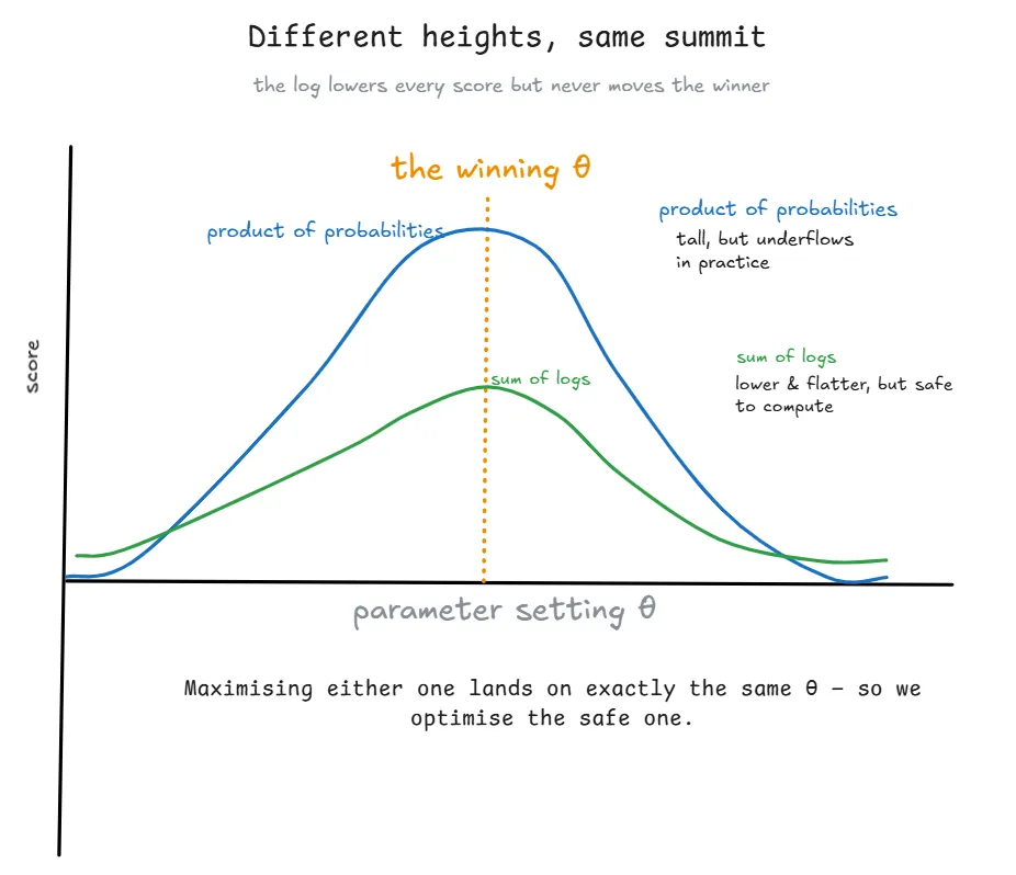
Second, and this is the property that answers the worry, the logarithm is monotonic: it never changes the order of things. If a > b, then log a > log b, always. This matters because training does not care about the actual value of the likelihood. It cares only about which setting of θ makes the likelihood largest. Since the logarithm preserves which value is largest, the winning θ is identical whether we maximize the product or its logarithm. Picture squishing a mountain range vertically: every peak gets lower, but the tallest peak is still the tallest. We have not moved the summit, only rescaled the heights.

$\arg\max_{\theta} \prod_i p_i \;=\; \arg\max_{\theta} \sum_i \log p_i$

So the logarithm is not a lossy shortcut. It is an exact re-expression, chosen for stability. The multiplication is still the true meaning underneath; the sum is just a safe way to carry it.

One last adjustment. By long convention we always minimize a cost rather than maximize a score. Maximizing Σ log pᵢ is the same as minimizing its negative, so we flip the sign. This is why the quantity is called the negative log-likelihood, and it is the general cost function we have been building toward.

$NN$

A Worked Comparison

It helps to see the order-preservation with numbers, because it dissolves a common confusion — the fear that summing the logs “mixes everything together” and loses track of the individual points. It does mix them, but the thing being ranked was never the individual points. It is the models.

Here, “two models” means the same one model at two different settings of θ — two snapshots of the same machine with its dials in two positions. Score each snapshot on the same three data points:

	example 1	example 2	example 3	product	sum of logs
Snapshot A	0.9	0.8	0.7	0.504	−0.685
Snapshot B	0.6	0.5	0.4	0.120	−2.120

Look only at the two summary columns. By product, A beats B (0.504 versus 0.120). By sum of logs, A also beats B (−0.685 versus −2.120). The winner is the same. That is the entire content of “the logarithm preserves order”: whichever snapshot scores higher by the product scores higher by the sum of logs. We never need to recover the individual pᵢ values, because the comparison we care about is between whole snapshots, and that comparison survives untouched.

This is also exactly what happens during training. Gradient descent walks θ from one snapshot to the next, always toward the better score. Because the product-score and the log-score rise and fall together as θ moves, walking uphill on one is identical to walking uphill on the other. Same summit, same path.

Cross-Entropy Is the Same Thing Under Another Name

One more piece of vocabulary, because the textbooks use it and it sounds more intimidating than it is. The negative log-likelihood we just built is, when written out over the data, exactly what is called the cross-entropy between the data and the model. Three names appear in the literature — maximum likelihood, negative log-likelihood, cross-entropy — and for our purposes they are three names for one idea: give high probability to what actually happened. Do not let the vocabulary multiply the concept. There is only one concept here.

A note for when you reach code: some libraries expose “cross-entropy” and “negative log-likelihood” as two separate functions that return different numbers. This is not a contradiction of what we just said. The mathematics is identical; the functions merely expect different inputs — one takes raw scores and applies the squashing-and-log step for you, the other assumes you already did that step yourself. Give each the input it expects and they agree.

Chapter 9: The Mean Squared Error, Derived

We now have a general recipe. It says: whatever your model’s output distribution is, the cost is the average negative log-probability it assigns to the real data. This chapter runs that recipe on one specific choice and watches the mean squared error — the loss we simply assumed in Part 1.1 — appear on its own.

The General Recipe

Written compactly, the cost is

$J(\theta) = -\,\mathbb{E}_{\,\mathbf{x},\mathbf{y}\sim \hat{p}_{\text{data}}}\ \log p_{\text{model}}(\mathbf{y}\mid \mathbf{x})$

Two symbols deserve a plain reading. The 𝔼[·] is just an average — go through every (x, y) example in the data, compute the thing inside, and average the results. The subscript p̂_data says the average is taken over your actual training set, the small hat marking that it is the finite sample you really have. So this 𝔼 is nothing more exotic than the (1/n)Σ you have used since Part 1.1, written in a more compact costume:

$\mathbb{E}_{\text{data}}[\,\cdot\,] = \frac{1}{n}\sum_{i=1}^{n}(\,\cdot \text{ for example } i\,)$

The minus sign in front is the one that turns “maximize probability” into “minimize a cost,” exactly as we arranged in Chapter 8.

One Choice: The Gaussian

The recipe does nothing until we say what distribution the model produces. We make the most natural choice for a continuous prediction: a Gaussian — a bell curve — centered on the network’s output f(x; θ). Written out, with its spread fixed at 1 to keep the algebra clean, the Gaussian is

$p_{\text{model}}(y \mid x) = \frac{1}{\sqrt{2\pi}}\ \exp\!\left(-\frac{(y - f(x;\theta))^2}{2}\right)$

Why the Gaussian and not some other curve? Because it is the natural description of “a prediction plus random noise.” When the noise on a measurement is the sum of many small independent disturbances — which is the usual situation in the physical world — a deep result called the central limit theorem says the combined noise tends toward a Gaussian shape, regardless of where the individual disturbances came from. The Gaussian is therefore not a wild guess; it is what noise usually looks like. It is also the choice that assumes the least beyond a center and a spread, and, as we will note shortly, it leads the model to predict the average outcome, which is what we usually want.

But keep in mind that this is a choice, and other choices are open to us. That fact becomes the punchline of the chapter after this one.

The Cancellation

Now we simply run the recipe. Take the logarithm of the Gaussian. The logarithm splits the two multiplied pieces into a sum, and — this is the mechanical heart of it — the logarithm undoes the exponential, because they are inverse operations. Whatever sits inside exp(·) comes straight back out:

The logarithm has one defining property we lean on constantly: $\log (A ⨉B )= \log (A) +\log (B)$

By applying this rule, we will obtain:

$\log p_{\text{model}} = -\frac{1}{2}(y - f(x;\theta))^2 \;+\; \log\frac{1}{\sqrt{2\pi}}$

Apply the minus sign from the recipe. This flips the sign of the whole line. The first term already carried a minus of its own from inside the exponential, so applying a second minus turns it positive — minus times minus is plus. The constant, which was positive, becomes negative:

$-\log p_{\text{model}} = \frac{1}{2}(y - f(x;\theta))^2 \;-\; \log\frac{1}{\sqrt{2\pi}}$

Finally, take the average over the data:

From this: $J(\theta) = \mathbb{E}\ [-\,\log p_{\text{model}}]$

Can get this now:

$J(\theta) = \frac{1}{2}\,\mathbb{E}_{\,\mathbf{x},\mathbf{y}\sim \hat{p}_{\text{data}}}\ \|\mathbf{y} - f(\mathbf{x};\theta)\|^2 \;+\; \text{const}$

Three things are worth naming. The ½ is not invented; it is the same ½ that sat inside the Gaussian’s exponent. The constant contains no θ at all, and since training only ever moves θ, a term with no θ can never change which θ wins — so we discard it without consequence. What survives, ½‖y − f(x;θ)‖², is exactly squared error. The mean squared error was hiding inside the general recipe the whole time. Choosing the Gaussian is what made it visible.

The Same Destination by a Different Road

It is worth stopping to notice what just happened, because you have now reached the mean squared error twice, from opposite directions, and both are legitimate.

In Part 1.1 you reached it bottom-up, by invention. You began by assuming squared error was a sensible way to measure a gap — the “so we invented one” move — wrote it down as the first equation, and then, in Part 1.2, did calculus on it to get gradient descent. That is the practical path: reach for a reasonable loss, then optimize it.

Here you reached it top-down, by derivation. You assumed almost nothing — only maximum likelihood — chose a Gaussian output, and derived squared error as the consequence. It was not the starting assumption; it was the conclusion.

Neither road is wrong, and the pair of them together is more valuable than either alone. The bottom-up road is faster and more intuitive, which is why it belonged in your first encounter. The top-down road is what turns the earlier invention into something justified: it explains why squared error was a reasonable thing to invent — it is the honest cost when your noise is Gaussian — and, more importantly, it reveals that squared error is only one item on a menu. The alternatives you might just as easily have invented in Part 1.1 — the absolute gap, for one — turn out to be the honest costs for other output distributions, each predicting a different statistic. That is where we go next.

What Comes in Part 1.4

We have done the hard half: the mean squared error is no longer an assumption but a result, derived from maximum likelihood and the choice of a Gaussian output. What we have not asked is whether it is the loss we should actually reach for.

Part 1.4 takes up that question. It shows that the choice of output distribution was exactly that — a choice — and that other choices give other costs, each predicting a different summary of the data. It also uncovers a problem hiding inside squared error: in the common case of a yes-or-no prediction, its gradient can fall silent at precisely the moment the model is most wrong. That failure, called saturation, is the reason practitioners so often prefer cross-entropy, and it is where the slope idea from Part 1 returns one last time.

The recipe is built. Part 1.4 is about learning to read the menu it produced.

Refrences

Goodfellow, I., Bengio, Y., & Courville, A. (2016). Deep Learning. MIT Press. Relevant chapter: Chapter 6 (Deep Feedforward Networks), Section 6.2.1 — Cost Functions. Available free at deeplearningbook.org.