The Math Behind Neural Networks, Part 1.2 — The Mathematics of Learning
May 24, 2026
A calm, sequential guide for anyone entering the field. The article is divided into smaller chapters to make it easier to understand.
Part 1.1 ended at a precise standing point: we had built a model, ŷ = wx + b, and we had a single number, the mean squared error, that told us how wrong that model was on average. What we did not have was a way to act on that number. A loss of 4.67 tells you the model is wrong; it does not tell you whether to push w up or down, and it does not tell you by how much. Part 1.2 is where that missing piece arrives.
We will introduce the derivative, derive the gradient of the loss with respect to w and b by hand, and then turn those gradients into an actual update rule through gradient descent. By the end of this part, the same three data points from Chapter 2 will be used in a full training example, and you will watch the loss fall step by step until the model converges to the true underlying relationship. The slope idea from Chapter 1 does not change. It simply gets sharpened into the tool that makes learning possible. Part 2 then takes that tool into networks with many layers.
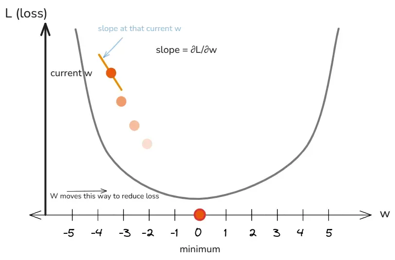
Chapter 4: The Derivative — The Slope of the Error
Why a Number Alone Is Not Enough
At the end of Chapter 3 we had a single number, L, that summarised how wrong the model was. With w = 1 and b = 0, the loss was 4.67. We know the goal is to make this number as small as possible. What we do not yet know is how.
A reader might suggest trying different values of w and b until the loss becomes small. With two parameters and a simple dataset, this is not impossible, but consider what it involves. Should w be increased or decreased? By how much? Should b be changed at the same time or held steady? A real neural network has millions of parameters, not two, and trying random combinations would take longer than the age of the universe.
The deeper issue is that the loss value, taken on its own, does not contain a direction. The number 4.67 tells you that you are wrong, but it does not tell you which way is less wrong. If I handed you only the number 4.67 and asked you whether to increase or decrease w, you could not answer. You would have to guess. The loss is a position, not a direction. These are two fundamentally different kinds of information, and you cannot extract one from the other by rearranging the same data. You have to ask a new question.
The Equations Have Been Building Toward This
To see why the derivative is the only thing that fits here, it helps to trace the logic of every equation we have written so far. Each one was forced into existence by a problem the previous one could not solve.
We began with the slope formula:
This worked perfectly when the data lay on a clean line, because the slope could be read off directly from any two points. But real data scatters, and the slope formula stopped applying. Different pairs of points gave different slopes, and none of them represented the whole dataset.
So we wrote a candidate line with unknowns to be learned:
This solved the previous problem by giving us a form for the line, but it created a new one. The values of w and b were unknown, and we had no way to evaluate whether a particular guess was good. The equation describes the model but contains no built-in measure of its quality.
So we invented one. We compared the prediction ŷ to the truth y across all data points and summarised the gap into a single number:
This solved the evaluation problem by giving us one number that measures total error. But it created the deepest problem of all, the one we are now standing at. The loss tells us that we are wrong but not which way to change w or b to be less wrong. The information we need is not contained in L. It is contained in how L changes when w changes, which is a different quantity entirely.
To extract that quantity, we need a new equation, one that asks the loss a question the loss formula on its own never asks: if w were slightly different, by how much and in what direction would L change? The mathematical object that answers this question is the derivative.
From Slope to Derivative
We already have the tool we need, in a simpler form. In Chapter 1, slope told us how y changes when x changes. The derivative is the same idea applied to a different setting. Instead of asking how y changes with x in the data, we now ask how the loss L changes with the parameters w and b in the model. The variables have changed, but the underlying question — how does one thing change as another changes? — is identical.
There is one refinement. The slope formula in Chapter 1 measured the rate of change between two distinct points. The derivative measures the instantaneous rate of change at a single point, which is what you get when those two points move infinitely close together:
This is not a different concept from slope. It is slope made precise. As the gap between the two points shrinks to zero, the slope of the line connecting them becomes the slope of the curve at that exact point.
Why the Derivative and Nothing Else
It is worth addressing directly why the derivative is the right tool here, rather than some other technique. The honest answer is that the derivative is not the only conceivable approach, but it is the only approach that works at the scale of a neural network.
Consider the alternatives. You could teleport to a random set of parameter values and check whether the loss is lower. This is random search, and with millions of parameters the number of locations to try is astronomical. You would never find a good model. You could try changing each parameter slightly in every direction and measure which change reduces the loss the most. This is finite differences, and it requires one full forward pass per parameter per step. A network with one million parameters would need one million forward passes for a single update, which is computationally hopeless.
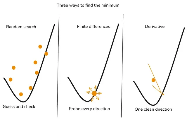
The derivative does something neither of these can. It uses the mathematical form of the loss function to compute the direction of steepest descent analytically, with no need to try moving in each direction first. Because of how calculus composes through the chain rule, all the derivatives in an entire neural network can be computed in roughly the same time as a single forward pass. This is the property that makes deep learning possible. Random search and finite differences fail because they treat the loss as a black box. The derivative succeeds because it exploits the structure of the loss directly.
There is a second reason that goes beyond efficiency. The derivative is exact in the limit. When the step size shrinks to zero, the derivative becomes the true instantaneous slope, not an approximation. Finite differences always carry an error that depends on how small your step is. The derivative has no such error. It is the mathematical object that perfectly captures how the loss responds to infinitesimal changes in the parameters, which is precisely the information needed to take the next step.
So when you ask why we use the derivative, the answer is not that we chose it from a menu of options. The answer is that the loss formula left exactly one piece of information missing — the direction of steepest descent — and the derivative is the only object that supplies that piece efficiently and exactly. There is no other equation that could occupy this position in the chain.
Deriving ∂L/∂w from MSE
We want to know: if I increase w by a tiny amount, does the loss go up or down, and by how much? To answer this, we compute ∂L/∂w, the partial derivative of L with respect to w. The word partial simply means that when we differentiate with respect to one variable, we hold all other variables fixed — even variables like b that we will also eventually learn.
Starting from the full loss with both w and b:
Step 1 — Identify the structure. The outer function is squaring, ( )². The inner function is the prediction error, (yᵢ − wxᵢ − b).
Step 2 — Apply the chain rule. The chain rule says: the derivative of a composition is the derivative of the outer function (evaluated at the inner function) times the derivative of the inner function. Since the derivative of u² is 2u, differentiating the outer function gives us 2 times the inner expression. Then we multiply by the derivative of the inner expression:
Step 3 — Differentiate the inner function with respect to w. Here yᵢ is a constant (it is data), and b is held fixed because we are taking the partial derivative with respect to w. The term wxᵢ differentiates to xᵢ, so:
Step 4 — Combine.
Where the 2/n Comes From
It is worth pausing on the 2/n in this final formula, because readers often wonder where the 2 came from. The 2 is not an arbitrary choice. It is the direct mechanical consequence of differentiating a square. When you differentiate any expression of the form , the result is — the exponent comes down in front and becomes a coefficient. This is one of the most basic rules of calculus, and it applies whenever a square is differentiated, regardless of what the inside expression is.
The 1/n that was already in front of the loss is not affected by the differentiation. It is a constant multiplier, and constants pass through derivatives unchanged. So when the squared term inside the sum produces a factor of 2 during differentiation, that 2 multiplies the existing 1/n, giving the 2/n you see in the final formula.
Deriving ∂L/∂b
The same process applies for b. The only difference is that differentiating (yᵢ − wxᵢ − b) with respect to b gives −1 rather than −xᵢ, because b has no x attached to it:
Both derivatives measure the slope of the loss surface. One tells you how the loss changes with w, and the other tells you how the loss changes with b. Together, they are the missing direction the loss formula could not provide on its own.
What Guidance Actually Looks Like
Once the derivative is computed, it produces a number with a sign and a magnitude, and both matter. If ∂L/∂w is positive, it means that increasing w would increase the loss, so to reduce the loss we need to decrease w. If it is negative, it means that increasing w would decrease the loss, so to reduce the loss we need to increase w. The sign of the derivative points us toward the correct direction. The magnitude of the derivative tells us how steep the loss surface is at this point, which is a proxy for how large a step we can confidently take.
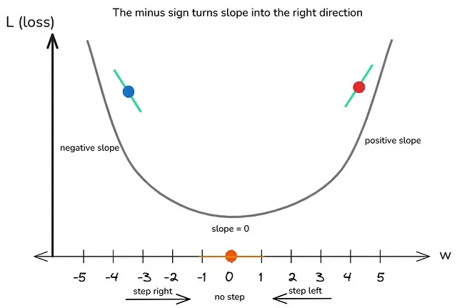
This is what is meant by training guidance. The derivative is not an abstract mathematical object here; it is a concrete instruction of the form “move w in this direction by roughly this much to reduce the loss.” Chapter 5 will convert that instruction into an actual parameter update, and you will see that the minus sign in the update rule is precisely the operator that converts the derivative’s measurement into the correct action.
Chapter 5: Gradient Descent — Following the Slope Downhill
The Update Rule
Once we have the gradients, we update each parameter by stepping in the direction that reduces the loss. This is gradient descent:
The symbol α (alpha) is the learning rate, a small number such as 0.1 that controls how large each step is.
Why Subtract the Gradient?
The minus sign in the update rule is doing real work, and it is worth understanding exactly what. The derivative tells us a measurement: it is positive when increasing the parameter would increase the loss, and negative when increasing the parameter would decrease the loss. But what we need is an action: we need to actually move the parameter in the direction that reduces the loss. Measurement and action are two different things, and the minus sign is the operator that converts one into the other.
Trace through both cases. If the derivative is positive, meaning the loss would grow as w grew, then subtracting a positive number from w causes w to shrink. The loss decreases as a result. If the derivative is negative, meaning the loss would shrink as w grew, then subtracting a negative number from w causes w to grow. The loss decreases in this case too. In both situations, the minus sign produces exactly the right movement to make the loss smaller. Without the minus sign, the update would push the parameters in the wrong direction, and the loss would climb instead of fall. The minus sign is the bridge between knowing the slope and using it.
A Full Training Example
Earlier we evaluated the loss at w = 1, b = 0 to have something concrete to measure. Here we restart from w = 0, b = 0 instead, so that the very first update is visible from the cleanest possible starting point: a model that predicts zero for everything.
Iteration 1 — Forward Pass (w = 0, b = 0)
| x | y | ŷ = 0x + 0 | Error (y − ŷ) | Error² |
|---|---|---|---|---|
| 1 | 2 | 0 | 2 | 4 |
| 2 | 4 | 0 | 4 | 16 |
| 3 | 6 | 0 | 6 | 36 |
Iteration 1 — Backward Pass
Iteration 1 — Update (α = 0.1)
Iteration 2 — Forward Pass (w = 1.867, b = 0.8)
| x | y | ŷ = 1.867x + 0.8 | Error² |
|---|---|---|---|
| 1 | 2 | 2.667 | 0.445 |
| 2 | 4 | 4.534 | 0.285 |
| 3 | 6 | 6.401 | 0.161 |
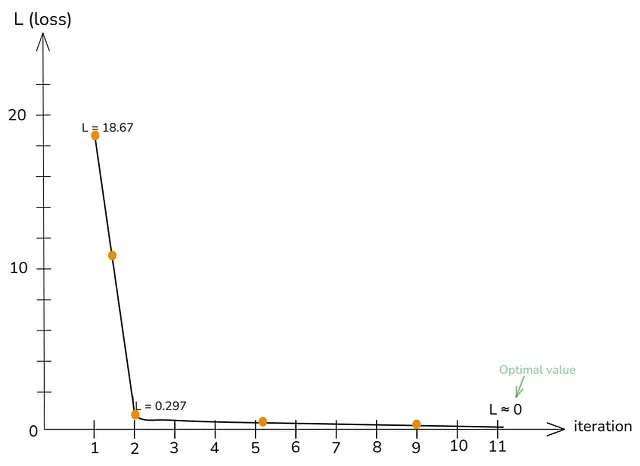
The loss fell from 18.67 to 0.297 in a single step. Both w and b are updated every iteration. The process continues until the loss approaches zero, at which point w converges to 2 and b converges to 0 — the true underlying relationship in the data.
Verifying the Gradient Direction
It is worth confirming that the gradient pointed the right way. We can check the loss at the starting point and at the true values directly:
| w | b | MSE Loss |
|---|---|---|
| 0 (starting point) | 0 | 18.67 |
| 2 (true value) | 0 | 0.00 |
The loss at w = 2, b = 0 is zero. The gradient correctly identified that increasing w reduces the loss. Nothing was assumed; it is verified by the numbers.
Chapter 6: The Unified Picture
How All Concepts Relate
Every concept covered here is answering the same underlying question: how does one thing change as another changes? The complete chain looks like this:
| Concept | What It Does | The Question It Answers |
|---|---|---|
| Slope | Measures rate of change between two points | How much does y change per unit of x? |
| Derivative | Instantaneous slope at a point | How does the output change at this exact input? |
| Linear Regression | Fits a line to data by learning w and b | What parameters minimise prediction error? |
| Error Function (MSE) | Measures how wrong the model is | How far is the prediction from reality? |
| Gradient | Derivative of loss with respect to each parameter | Which direction does the loss slope? |
| Gradient Descent | Uses gradient to update parameters | How should I adjust w and b to reduce loss? |
The Training Loop in Plain Language
A model trains by repeating four steps until the loss is small enough.
First comes the forward pass: using the current w and b to compute predictions ŷ = wx + b for every data point. Next comes the loss computation: calculating MSE to produce a single number representing total error. Then comes the backward pass: computing the gradient of the loss with respect to every parameter using the derivative formulas derived above. Finally comes the update: adjusting each parameter by stepping opposite to its gradient, scaled by the learning rate.
The model never knows the correct answer in advance. It starts blind, measures how wrong it is, uses the slope of that error to find the direction of improvement, and takes a small step. Repeat this process for as long as the loss keeps decreasing meaningfully, and a useful model emerges.
What Comes in Part 2
Everything in this article applies to a single linear layer: one weight, one bias, one equation. Real neural networks stack many such layers. But a critical problem arises when you do so: stacking linear layers produces another linear layer. No matter how many you add, the model remains fundamentally limited to linear relationships.
Part 2 introduces the solution: activation functions. These are nonlinear transformations applied after each layer that allow networks to learn curves, patterns, and complex decision boundaries. Part 2 will cover why linear layers stacked together are still just linear, what activation functions are and how they break linearity (ReLU, Sigmoid, Tanh), how the chain rule extends across multiple layers, what backpropagation actually computes step by step, and how gradient descent navigates high-dimensional space.
The slope equation never changes. The space just gets bigger.
Refrences
- Goodfellow, I., Bengio, Y., & Courville, A. (2016). Deep Learning. MIT Press. Relevant chapters: Chapter 4 (Numerical Computation, Section 4.3 — Gradient-Based Optimization), Chapter 5 (Machine Learning Basics, Section 5.1 — Linear Regression), Chapter 6 (Deep Feedforward Networks, Section 6.5 — Back-Propagation). Available free at deeplearningbook.org.