The Math Behind Neural Networks, Part 1.1 — The Mathematical Foundations
May 9, 2026
A calm, sequential guide for anyone entering the field. The article is divided into smaller chapters to make it easier to understand.
Deep learning can feel overwhelming at first. You encounter words like gradient, derivative, loss function, activation, and backpropagation, and it is rarely clear how they relate to each other or where they come from. This article builds the full picture from the ground up, starting from the simplest idea in mathematics, slope, and showing how that single idea grows into everything that powers a modern neural network. No step is skipped, and no formula appears without explanation.
By the end of Part 1.1, three concepts — slope, regression, and error — will form one continuous idea in your mind. You will understand what slope is and why it matters, what linear regression is trying to do, and what the error function measures. Part 1.2 then continues the journey with the derivative and gradient descent, the tools that turn a measurement of error into an actual improvement. Part 2 goes further still, introducing activation functions, multiple layers, and backpropagation, showing how everything here scales into deep networks.
Chapter 1: Slope — The Foundation of Everything
What Is Slope?
Slope answers one question: how much does the output change when the input changes?
If you drive 100 kilometers in 2 hours, your speed — the rate of change of distance with respect to time — is 50 km/h. That is a slope. If a ramp rises 3 meters over a horizontal distance of 6 meters, its steepness is 3/6 = 0.5. That is also a slope.
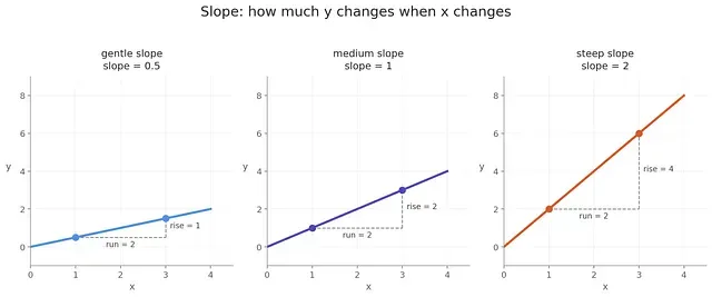
Formally, the slope between two points (x₁, y₁) and (x₂, y₂) is defined as:
This is called rise over run. The Greek letter Δ (delta) simply means change in.
A Concrete Example
Consider these three data points:
| x | y |
|---|---|
| 1 | 2 |
| 2 | 4 |
| 3 | 6 |
Taking points (1, 2) and (3, 6):
The slope is 2. Every time x increases by 1, y increases by 2. The relationship is perfectly linear and described by:
In real problems, however, we do not know the slope in advance. We have to discover it from data. That discovery process is called regression.
Chapter 2: Linear Regression — Learning the Slope from Data
From Knowing the Slope to Learning It
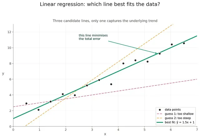
In Chapter 1 we had three neat data points that fell perfectly on a line, and we computed the slope directly with a formula. Real data is not like that, and the question this article exists to answer is how mathematics learns from data that does not fall on a clean line at all. When you collect measurements from the world — house prices against square footage, patient weight against medication dosage, temperature against electricity demand — the points do not land on a single clean line. They scatter. No two points give you the same slope, and no formula can hand you the answer.
This is where regression begins. Instead of computing the slope from two chosen points, we ask a different question: what is the single straight line that best represents all of the scattered points at once? That line will not pass through every point, but it will come as close as possible to all of them. Finding it means learning its slope and its vertical position from the data itself, rather than reading them off with a formula.
The Model Equation
To describe a line we still use the same form from Chapter 1, but with new names that reflect what each symbol now means in a learning context:
Here x is the input, the data you are given. The symbol ŷ (pronounced y-hat) is the model’s prediction — the value of y that the line produces for a given x. The letter w is the weight, which plays the same role as the slope m from Chapter 1; it is what you are trying to learn. The letter b is the bias, which is the vertical shift of the line, the same role played by the intercept in y = mx + b.
It is worth pausing on the distinction between y and ŷ. The value y is the true output in your data, the real measurement you collected. The value ŷ is what your model thinks the output should be for that same input. When the model is good, ŷ is close to y. When the model is bad, ŷ is far from y. The gap between them, y − ŷ, is the error, and it is what the next chapter is built around. Keeping these three quantities separate — the input x, the truth y, and the prediction ŷ — is essential for everything that follows.
What Is b and Why Does It Matter?
The bias b is not a fixed constant. It is a learnable parameter, just like w. Geometrically, w controls the steepness of the line and b controls where the line crosses the y-axis.
If the true relationship in your data is y = 2x + 5, then a model with w = 2 but b = 0 will be wrong by 5 for every single prediction. The network must learn b alongside w. Both are unknown at the start, and both are adjusted through training.
The Problem: How Do We Know Which Line Is Best?
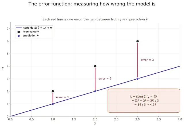
If we guess w = 1 and b = 0, our predictions for the data above are:
| x | y (actual) | ŷ = 1x + 0 | Error (y − ŷ) | Error² |
|---|---|---|---|---|
| 1 | 2 | 1 | 1 | 1 |
| 2 | 4 | 2 | 2 | 4 |
| 3 | 6 | 3 | 3 | 9 |
We need a single number that summarizes how wrong we are overall. That number is produced by the error function.
Chapter 3: The Error Function — Measuring How Wrong You Are
Mean Squared Error
The most common error function in regression is Mean Squared Error (MSE):
Breaking this down: for each data point, compute the difference between the actual value and your prediction, square that difference, and average over all points. Using our example with w = 1, b = 0:
This single number is what training is built around. Every choice we make from here on is in service of making it smaller. Before we move on, however, two pieces of this formula deserve real attention, because each of them is doing a specific job that the formula would not work without.
Why Divide by n?
The division by n turns a sum into an average. Without it, the loss would grow simply because you have more data, which would create a misleading picture of how well the model is performing.
Consider what happens without the division. If you have three data points and the squared errors are 1, 4, and 9, the total is 14. If you have thirty data points with the same average error per point, the total becomes 140. The model is performing equally well in both cases, but the loss number is ten times larger in the second case. This makes the loss meaningless as a measure of model quality, because its size now depends on dataset size rather than on how wrong the model is.
Dividing by n removes this dependency. The mean squared error gives you the average squared error per data point, which is a property of the model and the data together, not of how much data happens to be in your training set. With this normalisation, a loss of 4.67 means the same thing whether you computed it on three points or three million. You can compare losses across different datasets, across different training runs, and across different stages of training, and the numbers will be on the same scale.
There is also a practical reason that matters during training. The gradient of an unnormalised sum would also grow with n, which means the size of each update step would depend on dataset size. You would need to retune the learning rate every time you changed the amount of data. By dividing by n, the gradient stays on a stable scale regardless of dataset size, and a single learning rate works across many situations.
Why Square the Error?
Squaring serves three distinct purposes, and the most obvious one is only the first.
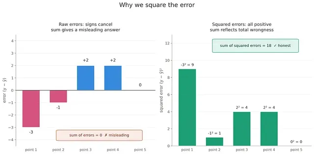
The first purpose is to remove the sign of the error. If the model predicts 5 when the true value is 3, the error is −2. If the model predicts 1 when the true value is 3, the error is +2. Both predictions are equally wrong, but if you simply added the raw errors, they would cancel and produce a total error of zero, which would falsely suggest the model was perfect. Squaring eliminates the sign, so both errors contribute positively to the loss.
The second purpose is that squaring penalises large errors more heavily than small ones. An error of 1 contributes 1 to the loss, but an error of 10 contributes 100. This is desirable because a model that makes one catastrophically wrong prediction is generally worse than a model that makes many slightly wrong predictions, even if the total absolute error is the same. Squaring builds this preference directly into the loss function. The model is pushed not just to be right on average, but to avoid being severely wrong on any single example.
The third purpose is the most important for training. The squared function is smooth and differentiable everywhere. The absolute value function, which is the most natural alternative for removing signs, has a sharp corner at zero where the derivative is undefined. Sharp corners cause real problems for gradient-based learning, and it is worth seeing exactly why.
What Sharp Corner at Zero Actually Means
Imagine the absolute value function plotted as a graph. It looks like a V: two straight lines meeting at a point. As you trace the line coming down from the left, the slope is constant at −1 the entire way. As you trace the line going up to the right, the slope is constant at +1 the entire way. But at the exact point where they meet — the bottom of the V — the slope suddenly jumps from −1 to +1 with no transition. There is no single number that describes the slope at that corner, because the slope on the left side is different from the slope on the right side. This is what mathematicians mean when they say the derivative is undefined at that point.
The squared function tells a different story. Its shape is a smooth U, and as you trace the curve from left to right, the slope changes gradually. On the far left, the curve is steep going down. As you approach the bottom, it flattens. At the very bottom, the slope is exactly zero. As you climb up the right side, it gradually steepens again. At every point along the curve, including the bottom, there is one well-defined slope, and that slope changes smoothly as you move.
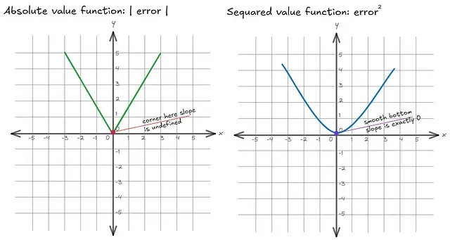
This matters for training because gradient descent works by reading the slope at the current position and moving in the opposite direction. If the loss function has a sharp corner, then at that corner the optimiser has no idea which way to move. The slope is +1 if you ask one way and −1 if you ask the other way, and these contradictory signals make it impossible to compute a clean update. The optimiser may oscillate, getting stuck bouncing back and forth across the corner without ever settling. The squared function avoids this entirely. Because the slope is well-defined and continuous everywhere, the optimiser always receives a clear, unambiguous signal about which direction to move and how confidently. As the model approaches the minimum, the slope naturally shrinks toward zero, which automatically slows the updates and lets the model settle smoothly into the optimal position.
Mean Absolute Error is still used in practice, particularly when robustness to outliers matters more than smooth optimisation. But for the kind of gradient-based learning that powers neural networks, the smooth bottom of the squared function is not a mathematical convenience. It is the property that makes clean convergence possible. There is one further reason MSE is particularly favoured: minimising it is equivalent to maximum likelihood estimation under the assumption of Gaussian noise, which connects the method to a deep foundation in probability theory.
With the loss in hand, we now face a deeper problem. We have a number that tells us how wrong the model is, but a number alone cannot tell us how to make the model better. To do that, we need something the loss formula does not provide on its own.
What Comes in Part 1.2
You now have three pieces of the picture: slope, regression, and a way to measure how wrong a model is. What is still missing is the most important piece of all — how the model actually improves. We have a number that tells us we are wrong, but a number alone cannot tell us which direction to adjust the weights. To turn measurement into action, we need a new tool.
Part 1.2 introduces the derivative and gradient descent. The derivative is the slope concept from Chapter 1 taken to its limit, and it is the one tool that can extract a direction from the error efficiently enough to train a real network. Gradient descent is what turns that direction into an update rule. The next article will cover why a number alone is not enough, how the equations from this article force the derivative into existence, where the 2/n in the gradient formula comes from, why we subtract the gradient instead of adding it, and a full worked training example showing the loss falling step by step.
The slope equation never changes. We are simply about to use it for something new.