The Math Behind Neural Networks, Part 0 — Where Deep Learning Comes From

A calm, sequential guide for anyone entering the field. The article is divided into smaller chapters to make it easier to understand.

Before any of the mathematics, it helps to know what we are building and why it has the shape it does. Newcomers to deep learning meet a wall of vocabulary — layers, weights, units, hidden layers, depth, features, backpropagation — usually with no sense of where any of it comes from or why it had to exist at all. This part answers that question first. It builds the whole picture in plain language, in the order the ideas actually depend on one another, so that when the mathematics begins in Part 1.1, every term already has a place to live. No idea is introduced before the one it rests on, and nothing is named without a reason.

By the end of Part 0, a single sentence will sit clearly in your mind: a neural network is a machine that learns its own features. You will know what the model is and the one equation that describes it, why it is built as a chain of layers, what those layers are made of, and why the field ended up needing hidden layers at all. This is only the beginning. What you are reading now is a map of the whole territory, drawn in plain language and with no mathematics yet. The parts that follow take their time — building each idea slowly and carefully from the ground up, one concept at a time — until everything named here, and much more besides, has been explained in full.

$NN$

Chapter 1: What a Neural Network Actually Is

The Model Everything Starts From

The foundational model of deep learning has one name and several nicknames. It is a feedforward neural network, also called a multilayer perceptron, or MLP for short. When people speak of “the quintessential deep learning model,” this is the one they mean. Almost everything else in the field — the systems that recognise faces, translate languages, or steer cars — is a variation or an extension of it. Understand this one model and you are holding the spine of the entire subject.

So what is it for? Always the same thing: to copy a rule we cannot write down.

Think of any task where an input should produce an output. A photograph should produce the label cat or dog. A house’s details should produce a fair price. A clip of speech should produce the words that were spoken. In every case there is a true rule connecting the input to the output — the rule your own mind applies without effort when it looks at a photo — but nobody can write that rule down as a clean formula. It is too intricate, and we do not fully understand it ourselves. So instead of writing the rule, we learn it from examples: we gather many inputs paired with their correct outputs, and we build a system that tunes itself until it reproduces them, in the hope that it has captured the underlying rule well enough to handle inputs it has never seen.

To talk about that system precisely, we first need a way to write it down. That is the one equation the whole field rests on.

The One Equation, Read Slowly

$y = f(x; \theta)$

Every symbol earns its place. Here x is the input — the photo’s pixels, the house’s details, whatever you feed in. The value y is the output the model produces — the label, the price, the answer you want back. The letter f is the function itself: the whole machine that turns x into y. And θ, the Greek letter theta, stands for the model’s parameters — the adjustable numbers that live inside it.

The semicolon is doing quiet but important work. It separates the two very different things f depends on. To the left of it, x is what arrives from the outside world. To the right, θ is what lives inside the model and can be changed.

Now the goal can be stated exactly. Somewhere out there is the true rule we wish we had; call it f*. We cannot build f* directly, so we build our own f and adjust θ until f behaves as much like f* as we can manage. That adjusting is training, and “as close as we can manage” is what people mean by the best approximation. Every technical idea in the rest of this series is, in the end, machinery for finding good values of θ. The next question is what f looks like on the inside. Why is it always drawn as a chain of boxes?

Chapter 2: The Shape of the Model

Why It Is a Network: The Chain

The function f is rarely a single step. It is built by sending the input through one small function, feeding that result into another, and so on down a line. Three such functions chained together look like this:

$f(x) = f_3(f_2(f_1(x)))$

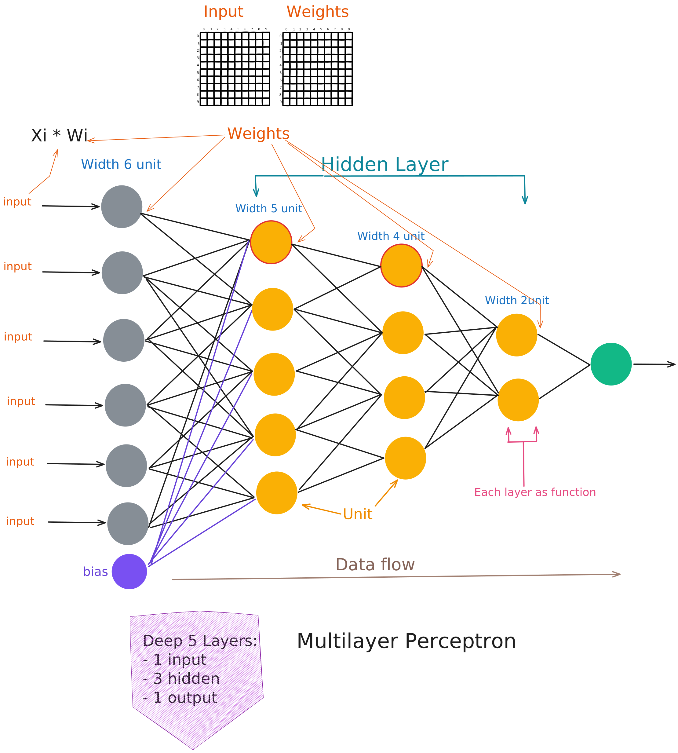
Read it from the inside out: the input x enters f₁; its result flows into f₂; that flows into f₃; and out comes y. Each function in the chain is a layer — f₁ is the first layer, f₂ the second, and so on to the last. Building something capable out of many simple pieces joined in sequence is exactly what the word network points at.

$NN$

The direction matters, too. Information only ever flows forward along this chain — in at one end, out at the other, never looping back on itself. That one-way flow is why these are called feedforward networks. Models that do loop back exist, and they are useful for other kinds of problems, but they are a separate story.

Notice that the chain has a length. That length carries the name the whole field is built on.

Depth: Where “Deep” Comes From

The number of layers in the chain is the depth of the model. A short chain is shallow; a long one is deep. That is the entire origin of the phrase deep learning — not depth of insight or meaning, but literally a long chain of layers stacked one after another. Each layer gets to work on what the layer before it produced, so a deeper chain can build up more elaborate results step by step. Depth is length, nothing more.

We have called each layer a function, but that leaves the obvious question unanswered: what is a layer actually made of? Open one up.

Inside a Layer: Units, and Why “Neural”

A layer is not one solid block. It is a row of small workers called units, all operating side by side. Each unit takes in many numbers (the outputs of the previous layer) and reduces them to a single number of its own. Collect the numbers produced by every unit in the layer, and together they form the layer’s output, ready to be passed to the next layer.

This is where the word neural comes from. A single unit is loosely modelled on a brain cell: a neuron also gathers signals from many others and produces one response of its own. The resemblance is deliberate but shallow — these units are far simpler than real neurons, and the aim was never to reproduce the brain, only to borrow one good idea from it. It is best to treat the biology as an inspiration, not a blueprint.

Two words for two directions, while we are here. Depth is how long the chain is, meaning how many layers it has. Width is how many units sit inside a single layer. A network can be deep, wide, both, or neither.

We said a unit combines many inputs into one number. But combines them how? That is where weights enter.

Why There Are Weights

Not every input to a unit deserves an equal vote. Some carry strong signal; others barely matter. So each connection feeding into a unit carries a weight (a number saying how much attention to pay to that particular input). The unit multiplies each incoming number by its weight, adds the results together (along with one extra adjustable number, the bias, which shifts the total up or down), and produces its output from that total.

$NN$

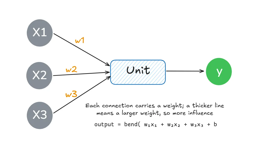
There is one more piece. After forming that total, the unit passes it through a small nonlinear step called an activation function. It is easy to overlook, but it does something essential: without it, stacking layer upon layer would collapse straight back into a single straight line, no matter how many layers you added. The activation function is the little bend placed inside every unit, and it is what lets a tall network describe curves instead of staying stubbornly flat. Part 2 gives it the full treatment; for now, just note that the bend is there and that it matters.

Here is the quiet payoff of all this. The weights and biases are the θ from our equation. When we said that training adjusts the model’s internal settings, this is precisely what we meant: training is the search for the right weight on every connection, so that the whole chain, from first layer to last, turns inputs into the correct outputs. A large network holds millions of these weights, and every one of them is learned rather than set by hand. So we have a chain of layers, each a row of weighted units, each unit ending in a small bend. One question is left, and it is the deepest of all: what should each layer actually compute? The training data gives a surprising answer.

Chapter 3: Where Deep Learning Actually Begins

What the Training Data Can and Cannot See

Training works by comparing the model’s output against the correct answer. For each example the data says, in effect: given this input, the final output should be this. The last layer — the output layer — is judged directly against that answer and pushed until it produces something close to it.

But notice what the data specifies and what it does not. It only ever pins down the output. It says nothing at all about what the layers in the middle should produce. No one labels the “correct” intermediate values, because no one knows what they ought to be. The middle layers are left to work out, entirely on their own, what to compute so that the output layer can succeed. Because their target is never shown anywhere in the data, these middle layers are called hidden layers — hidden not because they are secret, but because what they should do is never revealed to them.

Which raises the real question the whole field turns on. If nobody tells the hidden layers what to compute, what is it they are learning? The answer is features — and to see why features are the key, we have to return to the simplest possible model and watch it fall short.

Why We Need Features

Begin with the plainest model there is, a linear model — a straight line, or its higher-dimensional relative. Linear models are a pleasure to work with: quick to fit, stable, and completely predictable. Their weakness, though, is absolute. A straight line can only ever describe straight-line relationships. When the true pattern curves, or when two inputs only matter in combination rather than on their own, a line cannot bend to meet it, no matter how much data you pour in. Most problems worth solving are exactly this kind.

$NN$

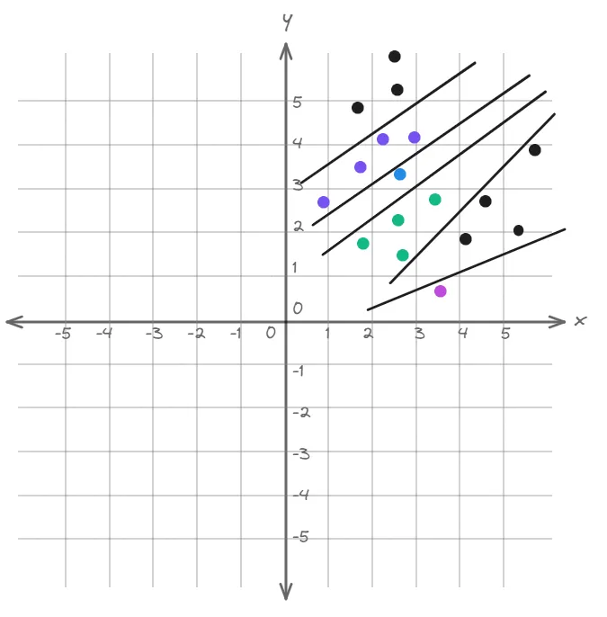
The way out is this: do not hand the raw input straight to the linear model. First transform the input into a richer set of quantities — features, sometimes called a representation — and let the simple model work on those instead. With the right features, a straight line drawn through them can capture something deeply nonlinear in the original input. Everything now hinges on a single question: where do the features come from? The field has tried exactly three answers, and the third is the one that gave birth to deep learning.

The first approach is to reach for a single, enormously flexible transformation that is tailored to nothing in particular, and apply it to every problem alike. The classic version expands the input into an effectively infinite collection of features — this is what a method like the RBF kernel does under the hood. With that many features to draw on, a straight line through them can fit any training set perfectly; the capacity is essentially unlimited. So why does it fail? Because fitting the training set was never the point — answering new inputs correctly is. A transformation this generic knows only one thing about the world: that inputs sitting close together should give similar outputs. It carries no real knowledge of the problem’s structure. In practice it memorises the training points and can only answer with confidence very near them, which means it needs to have already seen an example close to every future input — a hopeless demand in any rich, high-dimensional problem. It has unlimited power to fit and almost none to generalise.

The second approach is to design the features by hand. Human experts study the problem and craft the features themselves, out of their own knowledge of the domain. For decades this was how the field operated, and it could work well. But the price was brutal: each new task demanded its own specialists and years of trial and error, and features built for one problem — say, recognising speech — rarely carried over to another, such as recognising faces. Progress was measured in careers.

The third approach is to let the model learn the features for itself. Rather than fixing the transformation in advance or building it by hand, we let the model discover good features straight from the data, at the same time as it learns to use them. The human no longer has to find the exact right features — a nearly impossible task — but only to set out a broad, flexible family of possible transformations and let training choose a good one from within it. This asks the least of us and returns the most, and it is precisely what deep learning is.

The Equation You Will See in the Book

If you open the book itself, you will meet this third idea written compactly as

$y = f(x; \theta, w) = \phi(x; \theta)^\top w$

It looks dense, but it says exactly what we have just described, so let us read it in two halves. The inner part, φ(x; θ) — where φ is the Greek letter phi — is the feature transformation: it takes the raw input x and, using its own parameters θ, turns it into features. That transformation is the hidden layer. The outer part is nothing but our reliable linear model, now applied to those features instead of to x; w holds the weights that combine the features into the final answer, and the small raised ⊤ (a transpose) is just notation for the weighted sum we already know: line the features up against the weights, multiply each pair, and add. So the model carries two sets of adjustable numbers working together — θ, which shapes good features, and w, which reads those features out into an answer — and learning both at once is the whole game.

One point of notation deserves a pause, because it catches almost everyone. A moment ago we let θ stand for all of the model’s parameters, weights and biases alike. Here the same letter is used more narrowly: θ now names only the parameters inside φ, the ones that shape the features, while w is pulled out and given its own letter for the final weights that read those features into an answer. Nothing has changed about what they are. Both are still weights and biases, and w was always part of the larger θ; it has simply been lifted out and renamed so that the two jobs — building the features and using them — can be pointed at one at a time. When you see θ standing alone, read it as “everything”; when you see it beside w, read it as “everything except the final weights, which we are now calling w.”

Why Hidden Layers Exist

And now the picture closes. That learned transformation φ — the features the model invents for itself — is exactly what the hidden layers compute, and the bend we met earlier, the activation function inside each unit, is precisely what allows those features to be curved rather than flat. A hidden layer is the machinery that learns a good, nonlinear representation of the input without ever being told directly what that representation should be. This is why hidden layers exist at all, why they are called hidden, and why learning features is the beating heart of deep learning rather than a small detail off to the side.

The Whole Picture on One Page

Every term above, in the order it was introduced:

Term	Meaning
Model (f)	The function that turns an input into an output.
x, y	The input you provide and the output you want.
Parameters (θ)	The model’s adjustable internal settings.
Layer	One function in the chain.
Feedforward	Information flows one way, input to output, never looping back.
Depth	How many layers the chain has.
Unit	One small worker inside a layer; combines many inputs into one number.
Width	How many units a layer contains.
Weight	How much attention a unit pays to a given input.
Bias	An adjustable shift applied inside a unit.
Activation function	The small nonlinear bend inside a unit that lets the network curve.
Output layer	The final layer, judged directly against the correct answer.
Hidden layer	A middle layer that learns features on its own.
Features / representation	The useful quantities a hidden layer computes from the input.

What Comes in Part 1.1

Step back and look at what we now hold. A model is a function, y = f(x; θ), that tries to copy a rule we cannot write down. It is built as a chain of layers, and the length of that chain is its depth. Each layer is a row of units, and each unit takes a weighted sum of its inputs, adds a bias, and finishes with a small nonlinear bend; the number of units is the layer’s width. The final layer is checked directly against the correct answer, while the hidden layers in between are never told what to do — they must learn a useful representation of the input on their own. That act of learning the features, captured by φ(x; θ) in the equation above, is what separates deep learning from everything that came before it. All of that is the what.

What we have not touched is the how, and that is the entire journey ahead. Three questions remain open, and each has a precise answer waiting. First, how does a model measure exactly how wrong it currently is? That calls for a single number, a loss. Second, once it knows how wrong it is, how does it work out which way to nudge each of its weights to become less wrong? That is the job of the derivative and of gradient descent. Third, how can those nudges be computed efficiently across every layer of a deep chain at once? That is backpropagation, the algorithm that makes training a deep network practical at all, together with the activation functions that gave us the bends in the first place.

Part 1.1 begins the answer from the very bottom, with the simplest idea in all of mathematics: slope. From slope it builds linear regression, and from regression it builds the error function — the first precise measurement of how wrong a model is. Part 1.2 then turns that measurement into improvement with the derivative and gradient descent, and Part 2 scales the whole thing up into deep networks.

You now know what a neural network is. From here, we make it precise, one idea at a time.

References

Goodfellow, I., Bengio, Y., & Courville, A. (2016). Deep Learning. MIT Press. Chapter 6, Deep Feedforward Networks — chapter introduction (pp. 168–170). Available free at deeplearningbook.org.