Graph Laplacian: From Basic Concepts to Modern Applications

How a single matrix bridges discrete graph structures and continuous mathematical analysis.

Graph Laplacians stand at the intersection of spectral graph theory and modern machine learning, serving as a fundamental bridge between discrete graph structures and continuous mathematical analysis. This article explores three core aspects: the basic mathematical foundation of Graph Laplacians, their application in semi-supervised learning through smoothing techniques, and their role in spectral graph analysis through eigenvalue decomposition. By understanding these components, we’ll see how Graph Laplacians enable sophisticated applications in Graph Neural Networks (GNNs) and other modern machine learning architectures.

Let’s dive into the fascinating world of Graph Laplacians! It’s a powerful way to represent how things connect in a graph using matrices. If you’re into machine learning, especially semi-supervised learning, you’ll love this because it helps smooth out functions on graphs in really useful ways.

What Does It Really Depend On?

The Graph Laplacian builds on two key matrices. First up is the adjacency matrix (let’s call it A). Think of it as a map showing which nodes are connected to each other. If you have n nodes, you’ll get an n × n matrix. Here’s the cool part — you’re not just limited to 0s and 1s! While 0 means “no connection” and 1 means “there’s a connection,” you can actually use other numbers to show how strong the connections are.

Then we’ve got the degree matrix (D). It’s like a summary of how many friends each node has (or technically, how many edges connect to it). It’s a diagonal matrix, which means most spots are empty (zero), except for those special Dᵢᵢ spots that tell us about each node’s connections.

When we bring these together with L = D − A, we get the Laplacian matrix. The values might be positive or negative, but don’t worry about the negative ones — they’re actually super helpful for showing relationships between neighboring nodes!

Think of a social network where nodes are people and edges show how they’re connected. Let’s say we’re trying to figure out which users are into sports and which ones are into media. Here’s where it gets interesting; we only know this information for some users (that’s what makes it “semi-supervised” learning). We have a basic rule of thumb that says “If a group of nodes are connected, they are often, but not always, similar in characteristics.”

This is a simple example — let’s make it practical and compute the A and D matrices.

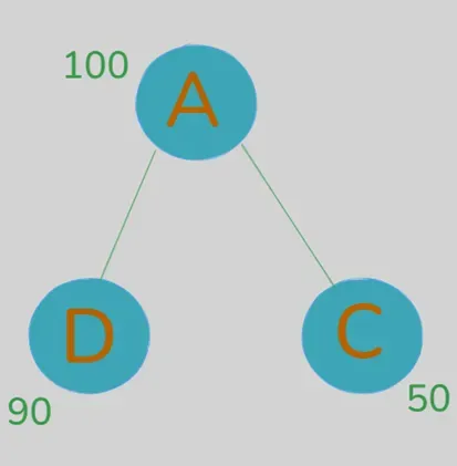
a) Get the adjacency matrix A:

A = [0 1 1]   // Node 1 connects to 2 and 3
    [1 0 0]   // Node 2 connects to 1
    [1 0 0]   // Node 3 connects to 1

b) Create the degree matrix D:

D = [2 0 0]   // Node 1 has 2 connections
    [0 1 0]   // Node 2 has 1 connection
    [0 0 1]   // Node 3 has 1 connection

c) Calculate the Laplacian matrix (L = D − A):

L = [ 2 -1 -1]
    [-1  1  0]
    [-1  0  1]

Calculating the Smoothing

The original law is graph Laplacian regularization:

ℒreg = Σᵢⱼ Aᵢⱼ ‖f(Xᵢ) − f(Xⱼ)‖²

But I will use a simpler law:

f_new(i) = (1−α)·f(i) + α·(average of neighboring nodes)

This formula is a variant of Laplacian smoothing, specifically Local Average Smoothing. It is widely used in semi-supervised learning, image processing, and graph-based learning.

Let’s solve it step by step for each node, using α = 0.5:

1. For node 1 (starting value = 100):

Neighbors are nodes 2 (50) and 3 (90)
Average of neighbors = (50 + 90)/2 = 70
f_new(1) = (1−0.5)·100 + 0.5·70
f_new(1) = 50 + 35 = 85

2. For node 2 (starting value = 50):

Only neighbor is node 1 (100)
Average of neighbors = 100
f_new(2) = (1−0.5)·50 + 0.5·100
f_new(2) = 25 + 50 = 75

3. For node 3 (starting value = 90):

Only neighbor is node 1 (100)
Average of neighbors = 100
f_new(3) = (1−0.5)·90 + 0.5·100
f_new(3) = 45 + 50 = 80

This gives us the smoothed values [85, 75, 80].

But using the Laplacian regularization term (ℒreg), these values aren’t the absolute minimum; they’re just a practical compromise between:

Keeping some of the original values (the (1−α) part)
Moving toward neighbor values (the α part)

Initial:         f'Lf = (100−50)² + (100−90)² = 2600
After smoothing: f'Lf = (85−75)²  + (85−80)²  = 125

The smoothing process reduced the total variation (penalty) from 2600 to 125, meaning:

Before smoothing:

Values: [100, 50, 90]
Penalty: 2600 (high variation)

After smoothing:

Values: [85, 75, 80]
Penalty: 125 (lower variation)

This shows how Laplacian smoothing makes node values more similar to their neighbors, reducing extreme differences. So, from these small differences between the nodes, the neural network can predict that the third node, which is not labeled, belongs to the same class as its neighbors, because the connected nodes have values close to it. This is the benefit of Laplace’s law.

Spectral Graphs

The Laplacian is also used in spectral graph theory — this is where we look at graphs through eigenvalues and eigenvectors. Don’t be intimidated by the fancy terms; think of eigenvalues as special numbers that tell us important things about the structure of the graph.

We find these values using:

det(L − λI) = 0,   where λ₁ ≤ λ₂ ≤ … ≤ λₙ

Each eigenvalue tells us something unique about the graph. For instance, if your graph is all connected in one piece, λ₁ will be 0. The number of times you get 0 as an eigenvalue tells you how many separate chunks your graph has!

Spectral graph theory is the study of graphs through the eigenvalues and eigenvectors of their matrices (especially the adjacency matrix and the Laplacian matrix), where the “spectrum” refers to the set of eigenvalues of these matrices.

For example, if we have 3 nodes, we will have three eigenvalues, and each one tells us something about the graph:

λ₁ = 0: Tells us about connectedness
λ₂: Tells us how well-connected the graph is
λ₃: Gives information about more complex structural properties

So, using the previous law, let’s find the eigenvalues of our graph. First, we construct (L − λI), where L is our Laplacian matrix and λ represents the eigenvalues we’re seeking. For our specific graph, this gives us:

|2-λ  -1   -1 |
|-1   1-λ   0 |
|-1   0    1-λ|

Next, we calculate the determinant of this matrix. The expansion leads to:

det(L − λI) = (2-λ)(1-λ)(1-λ) − (-1)(1-λ)(-1) − (-1)(-1)(0)
            = (2-λ)(1-λ)² − (1-λ) − 0
            = (2-λ)(1-λ)² − (1-λ)

Setting this equal to zero gives us our characteristic equation:

(1-λ)[(2-λ)(1-λ) − 1] = 0

Solving this equation reveals three eigenvalues:

λ₁ = 0
λ₂ = 1
λ₃ = 3

These eigenvalues tell us important things about our graph’s structure:

λ₁ = 0: This is normal and means your graph is one piece (connected)
λ₂ = 1: This small value warns that your graph is fragile — if you remove node 1, everything falls apart
λ₃ = 3: This larger value shows that node 1 is special — it’s doing most of the connecting work

In simple terms: your graph looks like a “Y” shape with node 1 in the middle holding everything together.

These eigenvalues are sometimes called the spectral values of the graph.

Why This Matters for Modern Machine Learning

All this theory becomes super practical when we look at Graph Neural Networks (GNNs). These networks need to understand how information flows between connected nodes, and guess what? The Laplacian’s properties are perfect for this! It helps the network figure out how to combine information from neighboring nodes while keeping the important patterns intact.

Wrapping It Up

So there you have it! The Graph Laplacian isn’t just some abstract math concept — it’s a powerful tool that helps us understand and work with connected data. Whether you’re trying to analyze social networks, build better machine learning models, or dive into graph theory, understanding the Laplacian gives you a solid foundation to work from. In the world of GNNs and graph-based machine learning, these concepts aren’t just theoretical; they’re the building blocks that make modern applications possible. The better we understand them, the better we can make our algorithms work for real-world problems!

Graph Laplacian: From Basic Concepts to Modern Applications

What Does It Really Depend On?

Calculating the Smoothing

Spectral Graphs

Why This Matters for Modern Machine Learning

Further Reading on Graph Laplacian Theory and Applications

Wrapping It Up